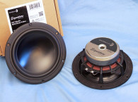
I tested the 7” ES180TI-8 midwoofer from Dayton Audio’s Esoteric Series of drivers. Starting with the frame, Dayton Audio used a nicely configured sixspoke cast-aluminum frame with narrow 9-mm wide spokes to minimize reflections back into the cone. The area below the suspended spider mounting shelf is almost completely open, resulting in effective cooling of the motor and the voice coil. For the cone assembly, Dayton Audio chose a rather stiff flat profile woven glass fiber cone with a 2.75” diameter convex woven glass fiber dust cap.
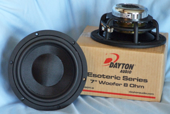
Compliance is provided by a nitrile butadiene rubber (NBR) surround, which is nicely designed with a shallow discontinuity where it attaches to the cone edge. Remaining compliance comes from a 4.5” diameter elevated black cloth spider.
The Dayton Audio ES180Ti’s motor design is well thought out and incorporates dual copper shorting rings (Faraday shields) and a neodymium ring magnet. FEA designed, the neodymium magnet motor uses a 3” (76 mm) diameter voice coil wound with rectangular copper-coated aluminum wire (CCAW) on a titanium former (with an ES180Ti designation). Motor parts include a polished chrome return cup for the neodymium ring magnet that incorporates a 35-mm diameter rear vent (with an open-cell foam dust cover) for additional cooling. Last, the voice coil is terminated to a pair of gold-plated terminals. In terms of physical appearance, this is very good-looking driver.
I used the LinearX LMS analyzer and the VIBox to create voltage and admittance (current) curves with the driver clamped to a rigid test fixture in free air at 0.3, 1, 3, 6, and 10 V. As with almost all 6.5” to 7” diameter woofers, 10-V curves are usually too nonlinear for LEAP to get a reasonable curve fit and usually have to be discarded. However, due to the ES180Ti’s linearity and high XMAX, I was able to use all the curves, including the 10-V curves.

As has become the protocol for Test Bench testing, I no longer use a single added mass measurement to determine VAS. Instead, I use the actual measured cone assembly mass (Mmd) supplied by the driver manufacturer, which was 26.2 grams for the ES180Ti. Next, I post processed the 10 550-point stepped sine wave sweeps for each ES180Ti sample and divided the voltage curves by the current curves (admittance) to derive impedance curves, phase added by the LMS calculation method. I imported them along with the accompanying voltage curves into the LEAP 5 Enclosure Shop software. Since most T-S data provided by OEM manufacturers is generated using either the standard model or the LEAP 4 TSL model, I used the 1-V free-air curves to create a LEAP 4 TSL parameter.
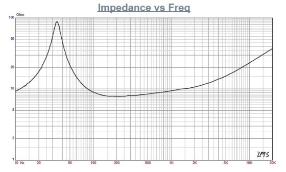
I selected the complete data set, the LTD model’s multiple voltage impedance curves, and the TSL model’s 1-V impedance curve in the transducer derivation menu in LEAP 5. Then, I created the parameters for the computer box simulations. Figure 1 shows the 1-V free-air impedance curve. Table 1 compares the LEAP 5 LTD, the TSL, and the factory published parameters for both of Dayton Audio’s ES180Ti-8 samples.
The ES180Ti-8’s LEAP parameter calculation results were very close to the published factory data. As usual, I followed my normal protocol and used the LEAP LTD parameters for Sample 1 to set up computer enclosure simulations. I programmed two computer box simulations into LEAP 5—one vented QB3 with a 0.4 ft3 volume tuned to 35 Hz with 15% fiberglass damping material and a Butterworth-type sealed enclosure with a 0.24 ft3 volume with 50% fiberglass fill material.
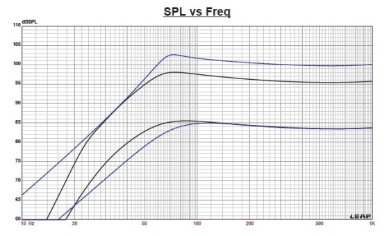

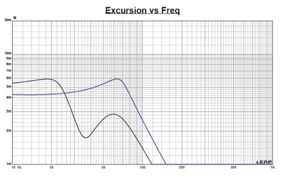
Figure 2 shows the ES180Ti-8’s results in the vented and sealed boxes at 2.83 V and at a voltage level sufficiently high enough to increase cone excursion to 61 mm (XMAX + 15%). This produced a F3 frequency of 48.8 Hz (F6 = 39.2 Hz) for the QB3 enclosure and –3 dB = 62 Hz (F6 = 50 Hz) with Qtc = 0.7. Increasing the voltage input to the simulations until the maximum linear cone excursion was reached resulted in 97 dB at 12 V for the QB3 enclosure simulation and 102.5 dB for a 22-V input level for the smaller sealed box. Figure 3 and Figure 4 show the 2.83-V group delay curves and the 12/22 V excursion curves. Because the vented box example reached maximum excursion at about 20 Hz, a steep 24 dB/octave high-pass active filter located at about 25 to 30 Hz would increase the power handling and output the vented box example by a substantial margin.
The ES180Ti-8’s Klippel analysis produced the Bl(X), KMS(X), and Bl and KMS symmetry range plots shown in Figures 5–8. This data is extremely valuable for transducer engineering, so if you don’t own a Klippel analyzer and would like to have analysis done on a particular project, Redrock Acoustics can provide Klippel analysis of almost any driver for a nominal fee.
Visit www.redrockacoustics.com for more information.
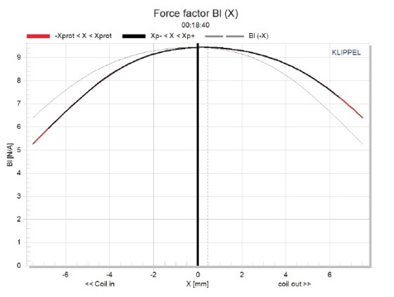
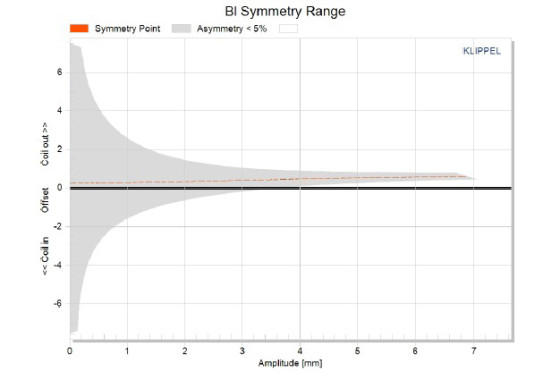
The ES180Ti-8’s Bl(X) curve is fairly symmetrical and moderately broad Bl curve for a 6.5” to 7” woofer (see Figure 5). The Bl symmetry plot’s curve shows a gradually increasing coil-out offset that reaches about 0.55 mm, the driver’s physical XMAX position, which is rather minor (see Figure 6).
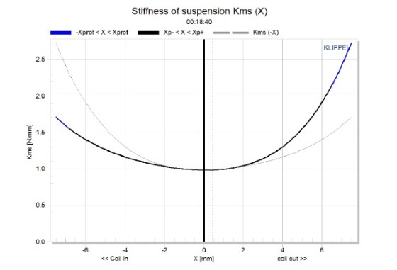
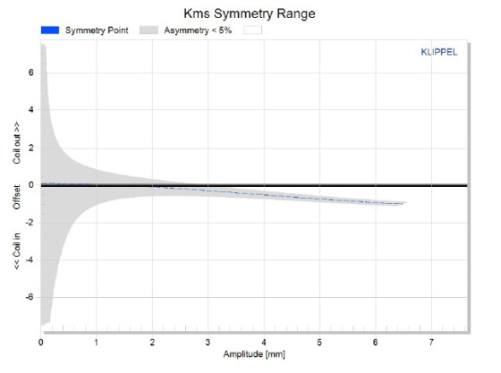
Figure 7 and Figure 8 show the ES180Ti-8’s KMS(X) and KMS symmetry range curves. The KMS (X) curve is definitely not as symmetrical in both directions as the Bl curve, and shows an increasing coil-in offset that gets to about 0.78 mm at the physical XMAX position, which is again relatively minor.
The ES180Ti-8’s displacement limiting numbers calculated by the Klippel analyzer were XBl at 82% Bl = 4.7 mm and XC at a 75% CMS minimum was 4.1 mm. For this Dayton Audio ES180Ti-8, the compliance is the most limiting factor for prescribed distortion level of 10%. If we use a less conservative 20% distortion criteria of Bl falling to 70% of its maximum value and compliance falling to 50% of its maximum value, the numbers would be XBl = 6.1 mm and XC = 6.1. Both numbers are greater than the ES180Ti-8’s physical 5.3-mm XMAX.
Figure 9 shows the ES180Ti-8’s inductance curves Le(X). Inductance will increase in the rear direction from the zero rest position as the voice coil covers more pole area. However, this does not occur because of the effective multiple copper inductive shorting rings. The result is a fairly minor inductance swing with inductive variation of only 0.03 to 0.05 mH from the resting position to the XMAXIN and XMAXOUT positions, which is good performance.
With the Klippel testing completed, I mounted the ES180Ti-8 woofer in an enclosure with a 15” × 8” baffle filled with damping material (foam). I used the LinearX LMS analyzer set to a 100-point gated sine wave sweep. Then, I measured the device under test (DUT) on and off axis from 300 Hz to 40 kHz frequency response at 2.83 V/1 m.

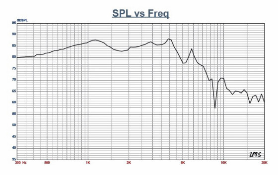
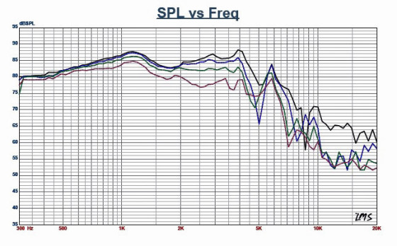
Figure 10 shows the ES180Ti’s on-axis response indicating a smoothly rising response to about 1.1 kHz, dropping about 5 dB to 2 kHz, and rising again to about 5 kHz where it begins its low-pass roll-off. Figure 11 shows the on- and off-axis frequency response at 0°, 15°, 30°, and 45°. The –3 dB frequency at 30° off axis relative to the on-axis SPL is about 2.4 kHz, suggesting a crossover between 2 to 3 kHz should be appropriate.
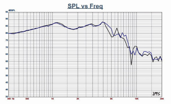
And finally, Figure 12 shows the ES180Ti-8’s two sample SPL comparisons, which is a close match throughout the operating range, up to 4 kHz.
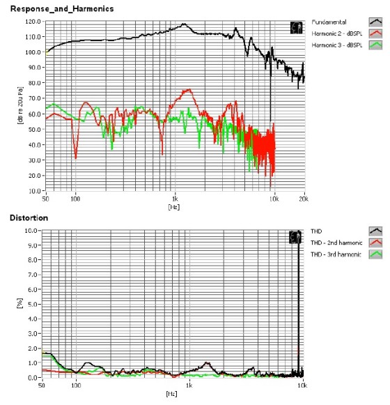
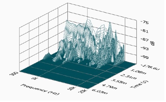
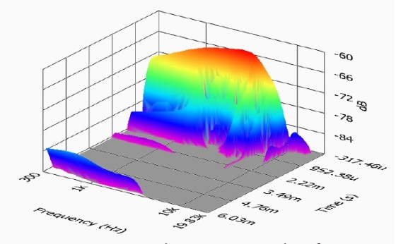
For the remaining tests, I again used the Listen SoundCheck software, the SoundConnext analyzer, and the SCM microphone (courtesy of Listen) to measure distortion and generate time-frequency plots. For the distortion measurement, I used a noise stimulus to rigidly mount the ES180Ti-8 in free air and set the SPL to 94 dB at 1 m (7.8 V). Then, I measured the distortion with the Listen microphone placed 10 cm from the dust cap. Figure 13 shows the distortion curves. I then used SoundCheck to get a 2.83 V/1 m impulse response and imported the data into Listen’s SoundMap Time/Frequency software. Figure 14 shows the resulting cumulative spectral distortion (CSD) waterfall plot. Figure 15 shows the Wigner-Ville plot (for its better low-frequency performance).
www.daytonaudio.com
This article was originally published in Voice Coil, December 2014