
Errors in the data used for these modeling programs will often lead to errors in the results the programs generate. In this article, we will detail some of the requirements to help assure good measurement data for use with loudspeaker modeling. It is also possible to use some of these loudspeaker modeling files to help optimize the design of crossover filters for the loudspeaker system. Since these modeling files have both on-axis and off-axis data, the effects of the crossover and equalization filters used for each pass band can be seen in the loudspeaker system’s overall directivity response. We will also show an example of this in a follow-up article.
While it is sometimes possible to measure a multitransducer loudspeaker system as a single radiating, full-range device, these measurements may be limited in their use. We certainly cannot use such measurements to help design the crossovers for the loudspeaker system. It is preferred that each separate pass band of a loudspeaker system is individually measured, when possible. These measurements are best performed with no filters in place. This allows the natural response of the drivers mounted in their enclosure to be captured.
There are some loudspeaker systems that do not allow for these separate pass band measurements. This can be a result of their design or operation. Each type of loudspeaker system must be evaluated as to how it acoustically functions. It is only possible to separately measure each pass band if each pass band actually radiates acoustical energy separately from the other pass bands in the loudspeaker.
Measurement Distance
The first thing we must do is to make sure the measurements are made in the far-field of the device we are measuring. Too often I hear people indicating they perform measurements at 1 m. After all, that’s the standard distance, right? WRONG! For all but very small loudspeakers a distance of 1 m is way too close to the loudspeaker. At that distance, we are most likely still in the near-field of the loudspeaker. In the device’s near-field, the frequency response can change as a function of distance from the device. In the far-field, the frequency response of the device itself will not change. Although air absorption can occur at higher frequencies when the measurement distance is relatively large, this is typically not a concern for the measurements we will perform.
The far-field of an acoustical radiator can be a function of both its size and the frequency (wavelength) that it radiates. In the low-frequency region, the distance at which the transition from near-field to far-field occurs is dependent only on the wavelength radiated (see Equation 1). From this we can see that our measurement distance needs to be at least one wavelength away from the device we are measuring.
[1]
Distance ≥ λ or Distance ≥ f/c
where λ is the wavelength, f is the frequency, and c is the speed of sound.
In the high-frequency region, the distance at which the transition from near-field to far-field occurs is dependent on both the size of the source and the wavelength radiated. For a line source, or a source that is like a line, the transition distance is given by Equation 2.
[2]
Distance ≥ h2 × f/2c
here h denotes the height of line-like radiator.
For non-line source devices (e.g., pistons, cone drivers, and horns), the transition distance is given by Equation 3. These devices have appreciable surface area and/or a relatively low aspect ratio (height/width).
[3]
Distance ≥ S × f/c
where S denotes the surface area of the radiator.
When evaluating S for a loudspeaker, we should often include the loudspeaker’s entire front surface, not just the surface area of the drivers themselves. This is necessary to account for the diffraction that occurs at the edges of the loudspeaker. These, too, are sources of radiation that are generally excited by woofers, midrange drivers, and dome tweeters.
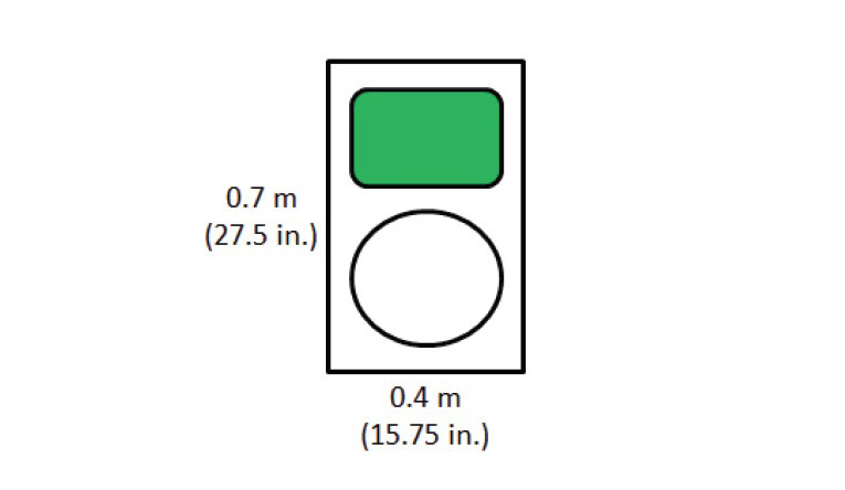
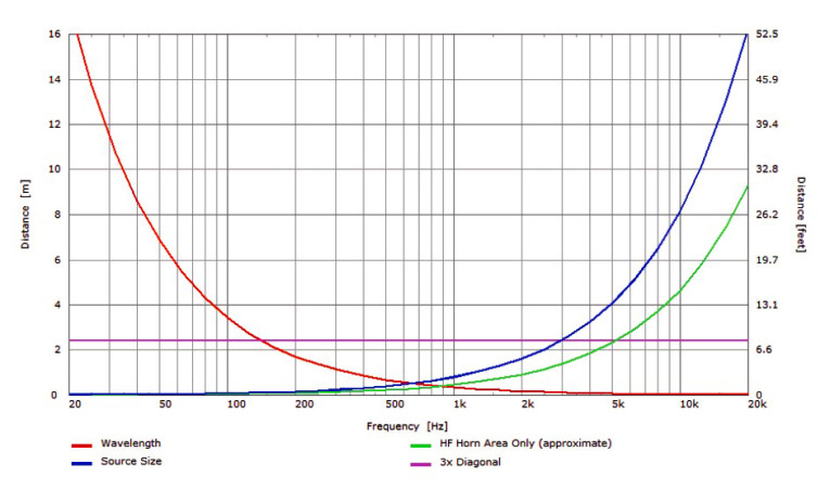
Let’s look at an example loudspeaker and see how far away we need to be for far-field measurements. We will use the loudspeaker shown in Figure 1. This loudspeaker has a height of 0.7 m (27.5”) and a width of 0.4 m (15.8”). This loudspeaker uses a horn-loaded high-frequency pass band and a direct radiator low frequency pass band. A rough rule of thumb often used for the measurement distance is 3× the baffle diagonal.
This would be about 2.4 m (7.9’) and is indicated by the purple line shown in Figure 2. The red curve is the minimum distance as defined by wavelength only. The blue curve is the minimum distance as defined by the source size (the entire baffle area). The green curve is the minimum distance required when we consider only the area of the high-frequency horn mouth. Since the horn has good directivity control at high frequencies, its radiation is not “illuminating” the baffle edges. We can typically use this distance in such cases.
We can see from the curves in Figure 2 that the 3× diagonal rule of thumb ensures we are in the far-field from about 150 Hz to above 5 kHz for this loudspeaker. If we need accurate data up to at least 10 kHz, we need to perform our measurements at least 4.7 m away from this loudspeaker.
Directivity and Angular Resolution[1]
When creating loudspeaker modeling files, we need to know how the loudspeaker system radiates sound into 3-D space. We must measure the off-axis radiation to characterize the loudspeaker’s directivity response. To do this accurately, our angular resolution must be finer than the lobes and nulls that the loudspeaker radiates. In other words, our spatial sampling interval must be finer than the spatial attributes of the directivity. This can be likened to the sampling frequency for an audio signal. If there are frequencies higher than one-half the sampling frequency in the signal, there will be aliasing in the result. Similarly, if our spatial (angular) sampling does not have at least two measurement points for a lobe or a null our measurement data will suffer from spatial aliasing.
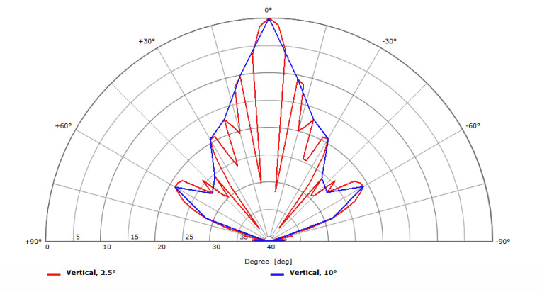
In Figure 3, we can see polar response plots for a line source device measured at 10° resolution and at 2.5° resolution. It is clear from looking at this graph that a spatial sampling of 10° is not sufficient to accurately characterize the directivity of this device. At some of measurement points for the 10° resolution data, the SPL is shown to be higher than it actually is. At other points, it is shown to be lower than it actually is.
So how can we know what angular resolution is required before we make our measurements? The off-axis angles at which nulls occur are related to the wavelength (frequency) radiated and the dimension of the source in the plane of interest. Mathematically, this relationship is shown in Equation 4.
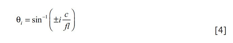
where f is the frequency, l is the length of the source in the plane of interest, i is a non-zero integer, and c is the speed of sound.
We can use this relationship to calculate the angular difference between two adjacent nulls. To assure we do not have undersampling errors (aliasing), we must have an angular resolution for our measurements of at least half the angle between these adjacent nulls (see Equation 5).
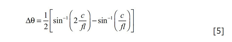
As an example, let’s say we want to accurately measure the vertical directivity up to 10 kHz for a ribbon driver that is 30 cm (11.8”) tall. At 10 kHz, the first and second vertical nulls occur at approximately 6.6° and 13.3°, respectively. One-half the difference between these angles is about 3.4°. The angular resolution of our measurements must be at least this. If we were to measure at an angular resolution of 2.5°, our data would be accurate up to about 13 kHz.
Directivity and Point of Rotation[2]
When performing off-axis measurements of a loudspeaker system, a point of rotation (POR) must be selected. This is the point about which the loudspeaker is rotated so that the measurement microphone is at the desired off-axis angle. If we are only interested in the magnitude of the off-axis frequency response, the location for the POR is not too important, within reason. However, if we will be using the measurement data for simulations to calculate the combined response of multiple devices, the location of the POR can be quite critical.
The reason for the importance of the POR has to do with the acoustic center (the point from which the radiation appears to originate) of the device under test (DUT). Ideally, we would like for the POR to be coincident with the DUT’s acoustic center. This is not always possible. A primary reason for this is that the acoustic center of an individual driver, much less a complete loudspeaker system, is rarely confined to a single location for all the frequencies radiated by the transducer or loudspeaker system. That is to say, the acoustic center can change location as a function of frequency.
If our measurements contain complex data (e.g., magnitude and phase), it is possible to deal with the POR not being coincident with the acoustic center, up to a certain point. The measured phase data can act as an error correction mechanism for the offset distance between the POR and the acoustic center of the DUT.
Note that this data must be the DUT’s actual measured phase response, not the phase response derived from the Hilbert transform of the magnitude only data. There is a limit to the offset distance that the phase data can effectively handle. This can generally be stated as a maximum of one-quarter wavelength at the highest frequency of interest.
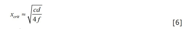
This limit for the offset distance, which has been termed the critical distance, manifests itself in the form of two different criteria. One is based on the measurement distance (the distance between the POR and the measurement microphone) and the other is based on the angular resolution used for the off-axis measurements. Each of these criteria are shown in Equation 6 and Equation 7, respectively. The lesser of these two values for the critical distance will be the governing value for the critical distance.
and
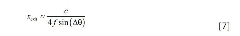
where c is the speed of sound, d is the distance from the POR to the measurement microphone, f is the highest frequency of interest, and Δq is the angular resolution for the measurements.
Let’s look at an example selection of the POR for a set of directivity measurements. We’ll use the same loudspeaker shown in Figure 1. This is a two-way loudspeaker system with a 12 dB/octave passive crossover at a frequency of about 1.2 kHz. We want to be able to accurately model this loudspeaker in clusters/arrays up to about 10 kHz. We will be measuring at a distance of 4 m, using an angular resolution of 5°. From this information, we can calculate the critical distances from the woofer’s acoustic center and the horn’s acoustic center. The radii for these distances will define spheres, shown here as circles, around the acoustical center of each radiator. The area where the circles (spheres) intersect is where the POR must be located for our measurements (see Figure 4).
The highest frequency of interest for the woofer is about 4.8 kHz. This is two octaves above the crossover frequency. If the crossover used higher order filters (steeper slopes), the woofer would not be radiating to as high of a frequency. Using the other values stated earlier gives us a critical distance (xcrit) of 0.268 m (10.6”) based on the measurement distance of 4 m and a critical distance of 0.206 m (8.11”) based on the angular resolution of 5°. Since the smaller value governs, the critical distance for the woofer is 0.206 m. The purple dashed circle shown in Figure 4 denotes this. It has a radius of 0.206 m, centered at the woofer’s acoustic center.
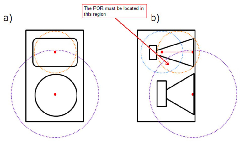
The highest frequency of interest for the high-frequency horn is 10 kHz, as this is the upper limit frequency for our modeling. Using the other values stated earlier gives us a critical distance (xcrit) of 0.186 m (7.32”) based on the measurement distance of 4 m and a critical distance of 0.098 m (3.68 in.) based on the angular resolution of 5°. Since the smaller value governs, the critical distance for the high-frequency horn is 0.098 m (see the orange dashed circle shown in Figure 4). It has a radius of 0.098 m, centered at the acoustic center of the high-frequency horn’s mouth. Note in Figure 4b the acoustic center can move from the mouth of the horn toward the throat of the horn at higher frequencies. The critical distance around this acoustic center closer to the horn’s throat is shown by the blue dashed circle. The entire range of locations for the high-frequency horn’s acoustic center must be considered.
The point of rotation for the off-axis measurements must be located where all of these circles intersect. Keep in mind that the POR and acoustic centers are actually defined in 3-D space so the circles represent spheres of the same radius as the circles shown.
Crossover Measurements
When the loudspeaker system’s individual pass bands are separately measured, with no filters in place, we also need to measure the crossover filters that will be used with the loudspeaker system so they can also be included in the loudspeaker modeling file.
It is a relatively straight forward process to measure the crossover outputs, but there are some things that must be considered.
These measurements must contain complex data, both magnitude and phase. If they are magnitude only, the resulting summation of the individual pass bands will not be correct. So a transfer function measurement must be performed. Here again, it is important that the measured phase response is used and not the Hilbert transform of the magnitude-only data. If an active or DSP-based crossover uses delay for some pass bands, this delay must be included in the phase response. Only the measured phase response will contain this. The Hilbert transform will just have the minimum phase component and not the complete phase response.
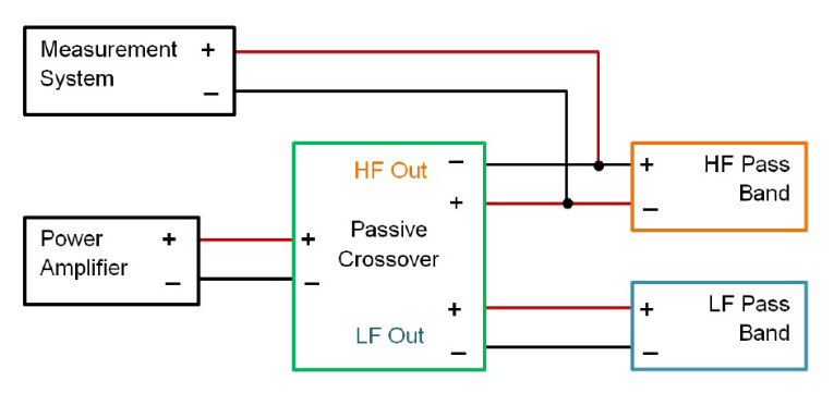
For measuring the transfer function of a passive crossover, it is best to measure at the input terminals of the driver(s) for each pass band. This gives an accurate representation of the signal present at the input of each pass band. Since a power amplifier is typically required to drive the input to the passive crossover take care when setting the output voltage from the amplifier. An rms voltage of 1 V is probably a good starting point. The inputs of most audio analyzers should be able to accommodate this voltage without any problems.
The polarity of the measurement data must be maintained compared to the signal’s polarity at the input to the loudspeaker drivers. That is to say, the measurement system’s positive lead should be connected to the driver’s positive input terminal and the measurement system’s negative lead should be connected to the driver’s negative input terminal. If the measurement system leads are not connected in this manner, the polarity of the transfer function measurement will be reversed. This can cause errors in the simulations using this data.
It is strongly recommended that only ground isolated, balanced inputs be used for measuring crossover outputs, particularly passive crossovers. It is not uncommon for passive crossovers to have an intentional polarity reversal for one or more of the outputs as part of the intended design. This is shown in Figure 5, where the high-frequency output of the crossover is reversed polarity. If a measurement system with a grounded, unbalanced input is used to measure a crossover output having reversed polarity, the positive output of the amplifier driving the crossover will be grounded. This will result in the amplifier’s output being shorted to ground. Not good!
Hopefully, this article has provided some ideas about how to make good measurements for use in loudspeaker modeling data files. Next, we will take a look at using loudspeaker modeling files to help design a crossover for optimum directivity response through the crossover region. Stay tuned. VC
Author’s Note: Some of the material presented in the referenced sections was originally published in presentations at Audio Engineering Society (AES) conventions and in the Journal of the Audio Engineering Society. For more details on these topics, please see the papers listed in References.
References
[1] S. Feistel and W. Ahnert, “Methods & Limitations of Line Source Simulation,” Journal of the Audio Engineering Society, Volume 57, No. 6, p. 379, June 2009.
[2] S. Feistel and W. Ahnert, “Modeling of Loudspeaker Systems Using High-Resolution Data,” Journal of the Audio Engineering Society, Volume 55, No. 7/8, p. 571, July/August 2007.
This article was originally published in Voice Coil, April 2017.