A recurring theme in my sound card article series (audioXpress, June 2015 to December 2015) was the software trade-off between versatility and feature set vs. complexity and learning curve. Inevitably, a versatile and powerful software package will be complex to use, and almost as inevitably, the user interface will be arcane and confusing. Simple and common features will be tucked away in unexpected places, the manual will have been written by a non-English speaking engineer, and tasks that should be smooth and rapid can take hours to get working the first time.
As time passes, the intrepid user will learn through repetition and hair-tearing and soon will be able to subconsciously operate the software, but the proficiency and familiarity will not be painless. Learning curves for complex software never resemble shallow ramps but always seem to be “Coyote and Road Runner” cliffs.
Among the software packages I mentioned was Multi-Instrument from Virtins Technology. It was complex. It was versatile. It was powerful. It drove me crazy. But in my usual prescient manner, I said, “I bet that a year from now, after I’ve gotten a greater comfort level, this will be my go-to choice for software.” And, I confess that this has indeed come to pass.
Virtins (a portmanteau of “Virtual Instrument”) is a Singapore-based company that sells a range of test and measurement software and hardware. Its principal products include USB-based digital storage oscilloscopes (DSOs), acoustic test and measurement systems, and vibration analysis systems. All of these products are comprised of a specialized hardware ADC/DAC module and a software system. The software system is also sold separately, suitable to be interfaced with a computer sound card, and is this article’s focus.
On my axis of complexity vs. versatility, the Virtins software lands far on the upper right. The array of features and flexibility is mind-boggling, but trying to get a comfort level with routine use takes some work, time, and struggle. No short review could possibly be comprehensive, but I’ll try to point out some useful features that you’re not going to find in competitive products.
The focus of this review will be a few (!) of the features that distinguish this software from other packages. All of the "normal” functions (e.g., distortion analysis, distortion vs. frequency, distortion vs. level, frequency response, etc.) common to other software are present. So, in the interest of space, I’ll glide by them relatively quickly, merely pointing out some extra capabilities within those functions that are useful and unusual.
allows control of the sound card outputs
with standard or custom waveforms.
Virtins divides the test and measurement process into three layers: sensor, hardware, and software. The sensor layer is the physical methods of acquiring a signal. It could be as simple as clip leads directly connecting a line level electrical signal to the sound card or something more complex such as a differential amplifier, a microphone and a preamp, or an accelerometer with signal conditioner. The output of this layer is a line level voltage.
The hardware layer is the data acquisition system, either a dedicated Virtins module, a National Instruments DAQmx card, or your sound card. Either way, there’s an analog-to-digital converter (ADC), and in most cases, a digital-to-analog converter (DAC) as well.
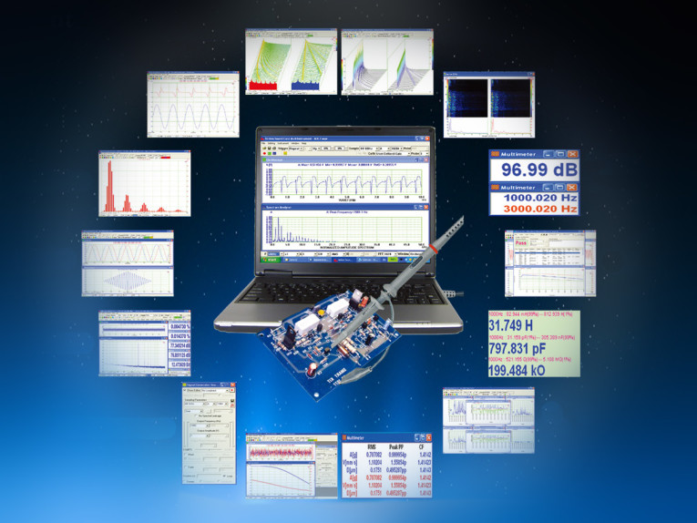
The software layer controls the acquisition and the output, then processes and displays the acquired data. Within the software layer, the Multi-Instrument program is set up as independent instrument modules, which can run and be displayed in any combination. This is analogous to using voltmeters, oscilloscopes, frequency meters, phase meters, distortion analyzers, and spectrum analyzers as stand-alone instruments, but with a much lower cost and much less dedicated bench space.
My Complications Have Complications
We get our first taste of complexity when we whip out our credit card. Virtins offers the Multi-Instrument in various level packages, with different optional modules, at varied prices. There’s six basic options, but the mixing and matching of package levels and modules is complex enough to require two lengthy tables on its website.
I’ll try to simplify your life: My recommendation is to spend the $200 it takes to buy the Pro version, mostly because it is the only level that allows use of Audio Streaming Input Output (ASIO) drivers rather than Windows Multimedia Extension (MME). There will be features that you’ll never use or don’t care about (it reminds me of having to buy some special rims on a car to get an automatic transmission), but I guarantee that you’ll find some uses you hadn’t previously imagined you needed, but suddenly can’t live without. Admittedly, this is more money than an extremely capable package such as ARTA costs, but it is considerably less than professional packages (e.g., Labview or MatLab).
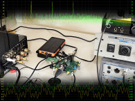
My Setup
As with most of the measurements in the sound card series, my test bed is an Hewlett-Packard desktop with an M-Audio Delta Audiophile 192 PCI sound card. I made up my own test leads, but Virtins sells various types as well.
to build up complex signals from selected
components.
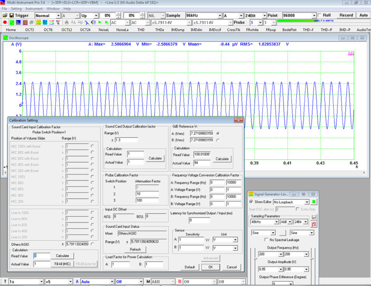
This step is actually pretty easy, but it will require some other calibrated meter (I used my trusty Fluke DVM) and a signal source (which can be the sound card’s output with the Signal Generator module running). Open the Calibration window found in the Settings menu overlaying the Oscilloscope module screen (see Figure 1). Set the signal source to a voltage high enough to register as 80% to 90% on the sound level bars in the Oscilloscope module screen.
The Oscilloscope screen will have a measured RMS voltage at the top of the display (shown as 1.8285 V in Figure 1). Enter this number in the Calculation box near the lower left corner of the Calibration screen. Now, measure the actual value with your voltmeter and enter the measurement result in the Calculation box. Click “OK” and you’re done. Use a test signal low enough in frequency that the AC reading on your voltmeter is accurate. If you’re not sure, 100 Hz will be safe.
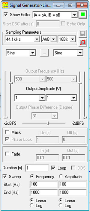
Signal Generator
The signal generator panel is small but busy (see Figure 2). Available signals include the usual sine, sawtooth, rectangle with variable duty cycle, white noise, pink noise, MLS, impulse, and step function. Additionally, the generator can provide a musical scale progression, as well as frequency sweeps for periodic signals. You can choose different signals independently for each channel, which can be useful in more complex measurements. It should be noted that the white noise and the pink noise are “true” continuous random signals rather than a limited random sequence, which is looped.
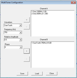
You can program your own custom signal as well, most simply with the Multitone option. In Multitone mode, you can specify various signals and add them together, outputting the sum into a selected output channel. For example, if you want to see the effect of adding low-level pink noise to a 1 kHz tone, or create a comb of different frequency, amplitude, and wave shapes, it’s a simple matter of choosing the component tone parameters (wave shape, amplitude, and phase) and adding it to the desired channel via a user interface, which pops up when you select the Multitone option on the signal generator panel (see Figure 3). It’s done iteratively. Choose the parameters of the signal’s component on the panel’s left side and hit the arrow in the middle to determine to which channel it’s sent.
One interesting feature in the panel is Mask. The Mask will zero out selected portions of the test waveform, selectable by the On and Off time parameters (e.g., when creating tone bursts). Let’s say you want 10 cycles of a 1 kHz burst repeated one per second. Set the record length for 1 second, then set the mask On to be 0.01 second, Off to be 0.99 seconds. You now have your tone burst.
The generator can also store, then read and output selected wav files. This can be handy to put together mixed waveforms (e.g., a sine tone burst followed by an impulse) or for using repetitive sections of a music selection as a test signal. Included in the package are a couple dozen standard test signals (e.g., various multi-tone signals for performing different intermodulation standard measurements).
Another neat feature is the option for “No Spectral Leakage.” If you click this option, the frequency is automatically adjusted to be centered in the nearest frequency bin, reducing the “skirts” at the base of the fundamental peak, which are a mathematical artifact of the sampling and transform process. This can be useful if you’re trying to resolve small peaks at frequencies close to the fundamental (e.g., power supply modulation).
The signal generator panel is also where a non-related but useful set of options are hidden — a virtual patch panel for signals. This appears at the top of the generator screen. Besides the expected options (e.g., sending signals to different combinations of channels, stereo, and mono), you also have the option of completely bypassing the sound card and doing a loopback in software at the Windows mixer level. That can be a useful way of learning how to use some of the Multi-Instrument features, and as Virtins points out, it can also be used for learning about various aspects of digital signal processing (DSP).
Multimeter
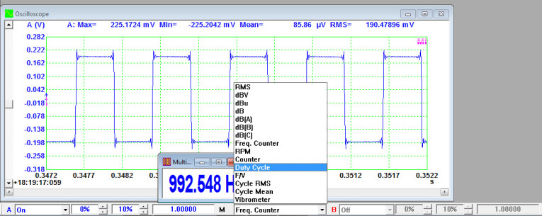
The most basic function in Multi-Instrument is called a Multimeter. It can measure frequency, voltage, level (in dBU, dBV, dB FS, and A, B, or C weighted), duty cycle, and counts. Figure 4 shows the Multimeter window and selectable options embedded in an oscilloscope window. In that screenshot, the Multimeter is reading the frequency of an applied square wave. I clicked on the menu pulldown to show the various other configurations available.
Derived Data Point Meter
This feature is basically the Multimeter on steroids. Besides reading and displaying the same sort of variables as the Multimeter, the Derived Data Point (DDP) meter adds in a few more—actually about 150 more! The displayed variables are updated with each acquired frame, so they are essentially real time. Up to 16 different DDP measurements can be simultaneously displayed.
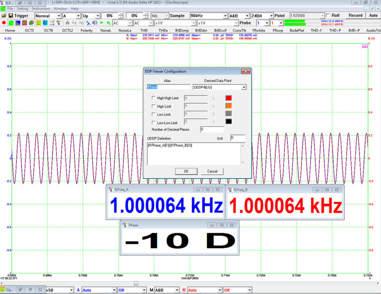
The derived part of the name refers to the ability to set up windows that can calculate custom measurements using a relatively simple syntax. Figure 5 shows an example.
I input a sine wave with a 10° phase shift between Channel A and Channel B (shown on the Oscilloscope screen). Using DDP, I chose two phase measurements, one for each channel. The phase shift is then the difference in phase between the two channels, so this calculation was entered into the User Defined Data Pont (UDDP) dialog box, the output assigned an alias (Phase), and the result displayed as a phase measurement. The user can define up to six different UDDPs.
Another DDP feature is its ability to set high and low limits giving visual warnings if a signal wanders outside of a user-specified range. This could be useful if the Multi-Instrument is used to monitor a process. It can also be helpful in troubleshooting situations, where you want to be warned if an over-voltage or over-current is being approached.
Oscilloscope
The oscilloscope module is pretty much what you’d think — a Digital Storage Oscilloscope (DSO), with bandwidth limited by the sound card’s sampling rate and input range. (Translation: It is not a substitute for a “real” oscilloscope.) As usual with DSOs, the sweep can be set as automatic or triggered, with level, slope, and delay all adjustable. The screen can display the usual Channel A, Channel B, and both simultaneously. It can also be set to display the sum, difference, and the product of the two channels. Curiously, there’s no option for ratio, but I’ll bet this shows up as a feature at some future time.
The oscilloscope module can record the output into a file on a continuous basis, with a 2 GB size limit. I haven’t tried using this feature as a digital recorder yet, but that will be coming soon! Where this capability differs from other systems is that the oscilloscope output can also be filtered using user-specified finite impulse response (FIR), infinite impulse response (IIR), or running Fast Fourier Transform (FFT). Built-in DSP includes low pass, high pass, band pass, and band stop filters.
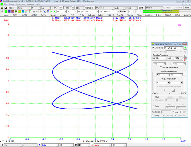
A simple and obvious feature that seems to be missing in other software packages is X-Y plotting, that is, a plot of the magnitudes of the A channel vs. the B channel during signal excitation. In the old analog oscilloscope days, phase and frequency measurements were often made using Lissajous figures (see Resources). Real-time Lissajous capability is selectable in the display options on the bottom of the screen (denoted as A|B).
Figure 6 shows a screenshot of the Lissajous pattern of 300 Hz and 500 Hz sine waves applied to Channel A and B, respectively. The trace can be used to determine frequency ratios and relative phase, as well as phase relationships between stereo channels. If a musical selection is used as a test signal, with Left fed to Channel A and Right fed to Channel B, a mono signal will result in a diagonal line. Stereo information will appear as a ”fuzzing” of the line.
I was fascinated by this feature, but a thought crossed my mind. Since we have a continuous display (or can do a one-shot display with infinite persistence), the Lissajous feature could be useful in looking at transfer functions (i.e., input vs. output).
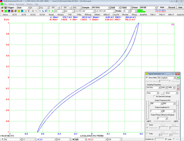
To test my idea, I rigged up a simple undegenerated common-source field-effect transistor (FET) stage with a gain of 3, then applied a 500 Hz sine wave to it. The A channel was connected to the applied signal, the B channel was connected to the FET drain (output).
Figure 7 shows the resulting trace. You can clearly see the square-law transfer function of the FET. This could be a nice way of visualizing nonlinearity in real time and possibly be the core of a curve tracer, with the addition of some fairly simple external electronics (sound cards cannot generally output DC). With a transducer attached to a speaker cone and the generator set to give an amplitude or frequency ramp, the function could also allow you to visualize nonlinearity of the speaker with increasing drive.
Spectrum Analyzer
As with most other measurement software packages, Multi-Instrument enables real-time amplitude and phase spectra to be calculated from the time domain signal using a FFT. There are a few enhancements, though. First, the number of window functions is vastly greater than in other measurement packages (55, count ‘em). If none of those suits your application, you can create your own. These are read into Multi-Instrument as wav files.
Another bit of extra flexibility is the FFT size. Multi-Instrument has the capability of a maximum of 4,194,304 data points per frame, which allows extremely fine frequency resolution, the trade off being acquisition and computation time. There are pre-packaged test plans to acquire spectra using various total harmonic distortion (THD) and intermodulation distortion (IMD) test signals.
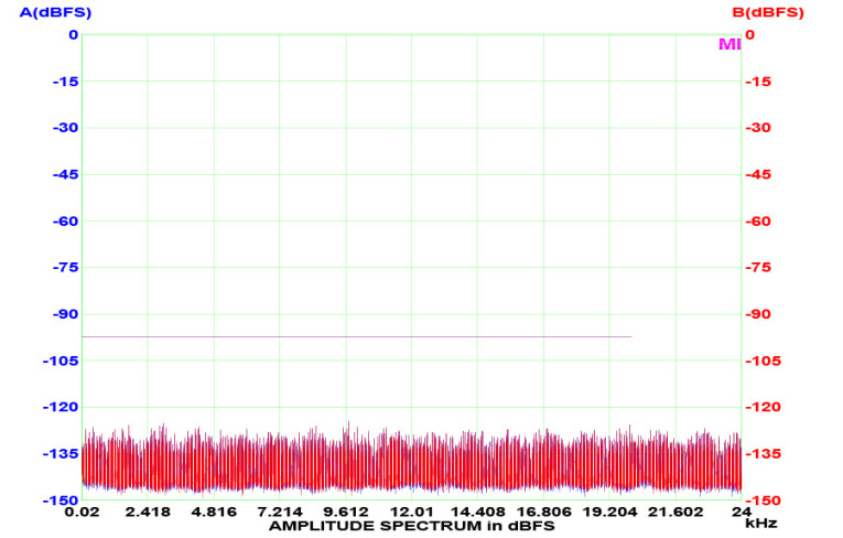
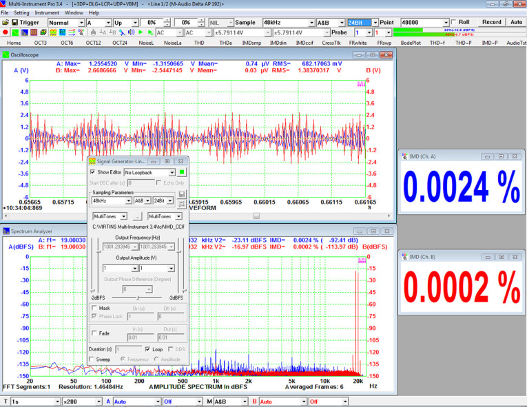
There’s also selectable options to acquire THD or IMD vs. power and THD vs. frequency, which are basic measurements for power amplifier characterization. Figure 8 shows an example of an IM measurement with 19 and 20 kHz tones. Note that besides the spectrum display, there are DDP boxes to give you the raw numbers, which is a handy feature in noise measurement. Generally, one has to calculate noise from the baseline using a summation of noise voltages in bins. This can be a tedious calculation if the noise floor isn’t flat. Multi-Instrument does this calculation with a menu option (NoiseL) and displays the result as a dotted line overlaying the noise floor (see Figure 9).
Other functions include frequency response (measured by either a swept tone or with white noise), cross-talk, and transfer function (acquired as a Bode plot or Gain and Phase plot). A useful and uncommon feature is the ability to measure correlation. The correlation between two signals is how closely they relate to one another as one of the functions is shifted through all possible values of time. If the two signals are applied to Channels A and B, the correlation R is defined as:
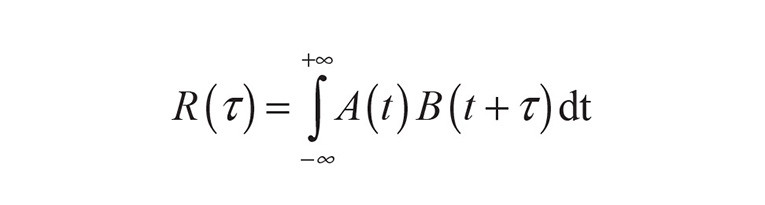
If Channels A and B are presented with the same signal, R is called autocorrelation. If they are different, R is called cross-correlation. The most useful thing about correlation functions is that they can be used to determine time delays between a stimulus and a response. In a simple case, an impulse is fed to a linear system and the output is measured. The delay is easily determined by comparing the timing of the output and the input signals, which can be done by eye.
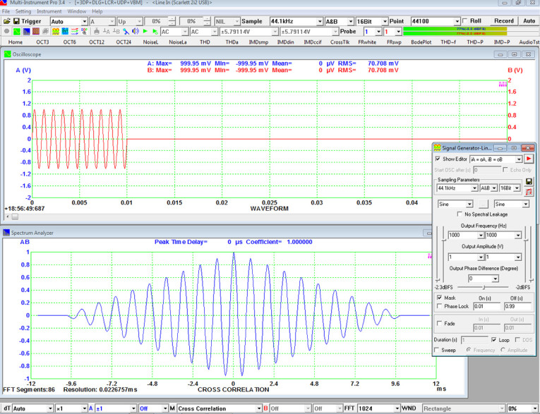
But what if the stimulus is a segment of white noise? Or the output signal is distorted, processed, or mixed with noise? Eyeballing is problematic. This is where the cross-correlation function can come in handy. It is evident that as the time delay between the signals at A and B approaches zero, the correlation will reach a maximum (see Figure 10). The specific example is a tone burst, but it could just as easily be a pseudorandom signal or an impulse buried in noise.
As a fun exercise (and a learning experience), Virtins has an instructional video showing how to use this function to measure the speed of sound, using white noise (see Resources).
Device Test Plan
If the user wants to configure Multi-Instrument to automatically run a series of tests, the Device Test Plan function can be used to program the desired test signals, the measurements, and the Pass/Fail criteria. The capability here is high enough that an entire article could be written on using this feature to create a virtual Automatic Test Equipment function.
Multi-Instrument can also be used to control external test equipment using standard protocols such as ActiveX and Virtins’s proprietary application program interfaces (APIs). This will primarily be used in professional quality assurance operations, but it could also come in handy for the amateur who wants to match or sort transistors or FETs for multiple variables (e.g., Idss and gm).
The software includes about 100 pre-written Device Test Plans that cover a range of common measurements. These can be run individually or as a specified series.
Summing Up
Multi-Instrument is a stunningly versatile and capable software package. It is far more complex and difficult to use than most hobbyist-oriented software (e.g., ARTA or AudioTester) and costs significantly more. But the price is reasonable compared to professional packages, and the capabilities far exceed the simpler software. The simpler and less expensive software will likely take care of 80% of your needs, but once you have climbed the learning curve for Multi-Instrument, your measurement power will be an order of magnitude greater.
I will confess that writing this review was delayed again and again as I’d discover a new feature or a new way to use existing ones. I still think that I haven’t used more than 5% of Multi-Instrument’s capability. My procrastination was aided by an excellent set of application videos that Virtins has produced for its YouTube channel.
The videos explain basic concepts and walk you through science-fair-level demos (e.g., using crosscorrelation functions to measure the speed of sound), which are good ways of learning basic measurement methods. They are also useful for discovering more of the software capabilities than are first evident. The production values of the videos are good, but the “Mr. Roboto” synthetic voice-overs are rather jarring. Overall, this software is highly recommended. aX
This article was published in audioXpress, March 2016.
About the Author
Stuart Yaniger has been designing and building audio equipment for nearly half a century, and currently works as a technical director for a large industrial company. His professional research interests have spanned theoretical physics, electronics, chemistry, spectroscopy, aerospace, biology, and sensory science. One day, he will figure out what he would like to be when he grows up.
Resources
“Lissajous Curves,” Wikipedia - https://en.wikipedia.org/wiki/Lissajous_curve
“Measuring Phase Shift,” YouTube - https://www.youtube.com/watch?v=L78tdU9wPVc
“Overview of Multi-Instrument,” YouTube - www.youtube.com/watch?v=msx5envAgGw
“Using Cross-Correlation to Measure the Speed of Sound,” YouTube - www.youtube.com/watch?v=7u1nSD0RlwY
“Using Cross-Correlation to Measure Time Delay,” YouTube - www.youtube.com/watch?v=L6YJqhbsuFY