This motor assembly uses a neodymium slug and a 1.5” diameter return cup that incorporates a T-pole. The cone assembly of this clever design is comprised of a flat cone made from an aluminum honeycomb layer sandwiched between two layers of woven glass-fiber cone material.
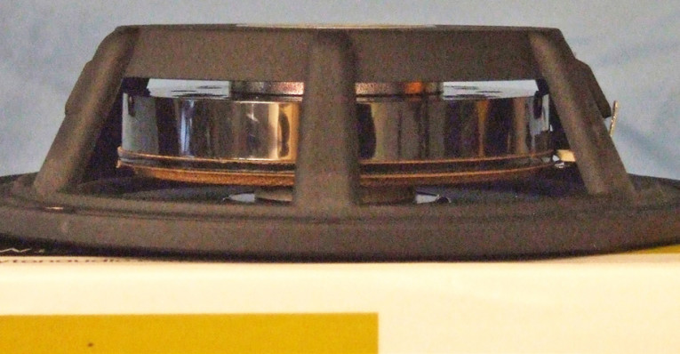
Suspension is provided by an S-shaped nitrile butadiene rubber (NBR) surround and two cloth spiders. The twin spiders are mounted on a plastic shelf that is vented on the back side with 12 4-mm diameter peripheral holes for cooling. They also enable the driver to be mounted flush to the cabinet’s back wall. Driving the assembly is a 1.25” diameter four-layer voice coil wound with round copper wire on a Kapton former, terminated to a pair of solderable terminals.
I commenced the LW150-4’s analysis using the LinearX LMS analyzer and VIBox to create voltage and admittance (current) curves with the driver clamped to a rigid test fixture in free-air at 0.3, 1, 3, 6, and 10 V. I had to discard the 10 V as they were too nonlinear for LEAP Enclosure Shop to get a good curve fit. As has become the protocol for Test Bench testing, I no longer use a single added mass measurement to determine VAS, but use the actual measured cone assembly mass (Mmd) supplied by the driver manufacturer, which was 21.9 grams.
Next, I post-processed the eight 550-point stepped sine wave sweeps for each LW150-4 sample and divided the voltage curves by the current curves (admittance) to derive impedance curves, phase added by the LMS calculation method. I imported the data, along with the accompanying voltage curves, to the LEAP 5 Enclosure Shop software.
Since most T-S data provided by the OEM manufacturers is generated using either the standard model or the LEAP 4 TSL model, I created a LEAP 4 TSL parameter set using the 1 V free-air curves. I selected the complete data set, the multiple voltage impedance curves for the LTD model, and the 1 V impedance curve for the TSL model in the transducer derivation menu in LEAP 5. Then, I created the parameters for the computer box simulations.
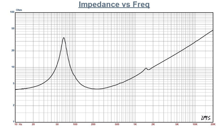
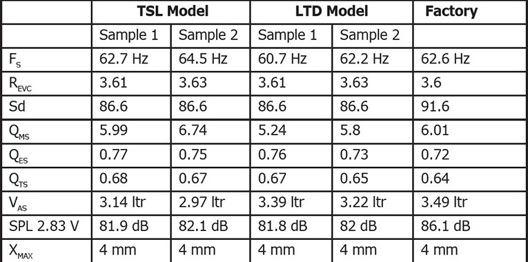

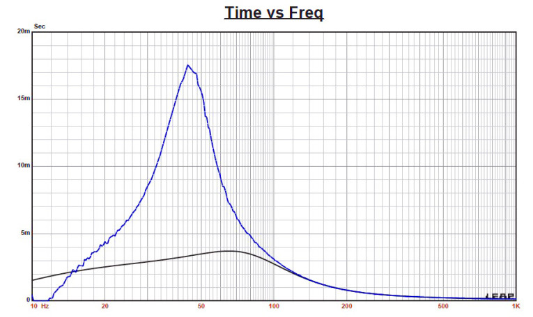

Figure 1 shows the LW150-4’s 1 V free-air impedance curve. Table 1 compares the LEAP 5 LTD, TSL, and factory published parameters for both of Dayton Audio LW150-4 samples. The LW150-4’s LEAP parameter calculation results were close to the published factory data, except for the Sd and the 2.83 V/1 m sensitivity. The Sd that I used included 50% of the surround, and was 10.5 cm. The Dayton specification is based on a more liberal 10.8 cm, which is not really significant and does not account for the difference in sensitivity. Ignoring this and following my normal protocol for Test Bench testing, I set up computer enclosure simulations using the LEAP LTD parameters for Sample 1.
I programmed two computer box simulations into LEAP 5, both recommended by Dayton Audio. The first was a sealed enclosure with a 0.24 ft3 volume with 50% fiberglass fill material, and a vented box with a 0.33 ft3 volume tuned to 40 Hz with 15% fiberglass damping material.
Figure 2 shows the LW150-4’s results in the sealed and ported boxes at 2.83 V and at a voltage level high enough to increase cone excursion to 4.6 mm (XMAX + 15%). This produced a F3 frequency of 73 Hz (F6 = 58 Hz). QTC = 0.77 for the sealed enclosure. –3 dB = 48 Hz (F6 = 43 Hz) for the vented alignment.
Increasing the voltage input to the simulations until the maximum linear cone excursion was reached resulted in 99 dB at 14 V for the closed box enclosure simulation and 102 dB for the same 14 V input level for the larger vented box. Figure 3 shows the LW150-4’s 2.83 V group delay curves. Figure 4 shows the LW150-4’s 14 V excursion curves. Note that the vented box example reached 4 mm of excursion at about 40 Hz so adding a steep 24 dB/octave high-pass active filter located about 25 to 35 Hz would prevent over excursion and distortion for vented box example by a substantial margin.
The LW150-4’s Klippel analysis produced the Bl(X), KMS(X), and Bl and KMS symmetry range plots shown in Figures 5–8. (Our analyzer is provided courtesy of Klippel GmbH. The analysis is performed by Pat Turnmire, of Redrock Acoustics. This data is extremely valuable for transducer engineering, so if you don’t own a Klippel analyzer and would like to have analysis done on a particular project, visit www.redrockacoustics.com.)
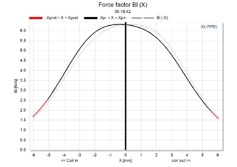
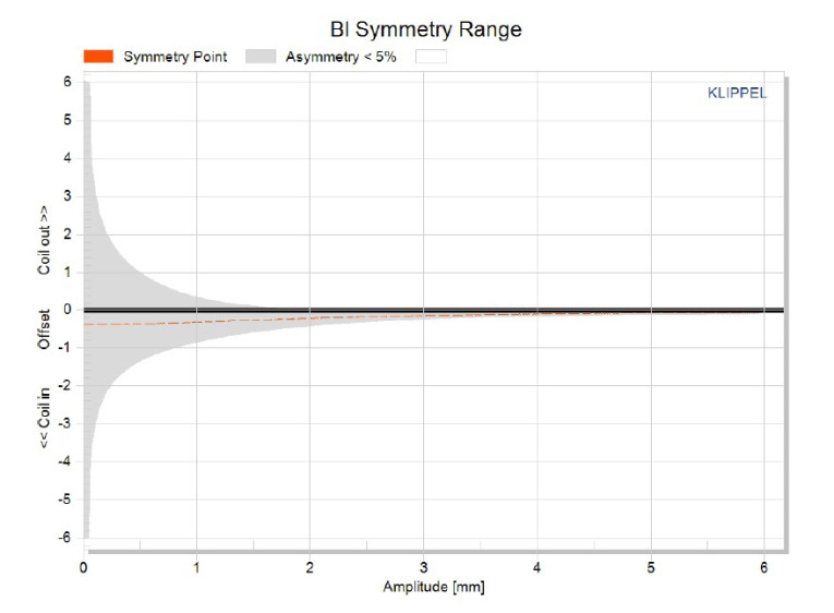
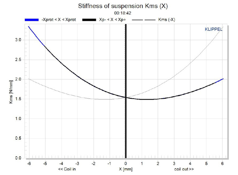
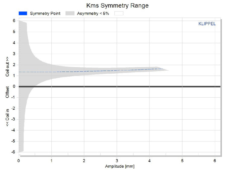
Figure 5 shows the LW150-4’s Bl(X) curve is very symmetrical and fairly typical for a short XMAX driver. Figure 6 shows the Bl symmetry plot, and this curve shows a really insignificantly small 0.2 mm coil-in offset once you reach the area of high certainty (around 2 mm of excursion). Figure 7 and Figure 8 show the LW150-4’s KMS(X) and KMS symmetry range curves. The KMS(X) curve is definitely not as symmetrical in both directions as the Bl curve. It shows a forward bias coil-out offset that gets to about 1.5 mm at the physical XMAX position. This does not create a subjective problem and like guitar speaker with a small forward bias, produces some “warm” sounding second harmonic distortion.
The LW150-4’s displacement limiting numbers (calculated by the Klippel analyzer) were XBl at 70% Bl = 3.3 mm and for the crossover (XC) at 50% CMS minimum was greater than 5.1 mm, which means that the Bl is the most limiting factor for prescribed distortion level of 20%.
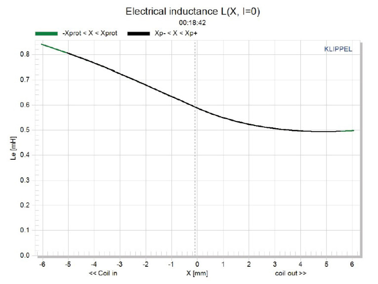
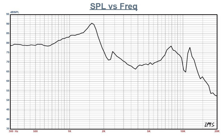
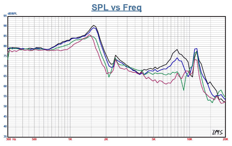
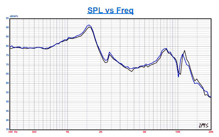
Figure 9 gives the LW150-4’s inductance curves Le(X). Inductance will typically increase in the rear direction from the zero rest position as the voice coil covers more pole area which is what is happening here. However the inductive swing is small, 0.174 mH from rest to the XMAX coil-in position, and 0.094 mH from the rest position to the 4 mm XMAX coil-out position.
I mounted the LW150-4 in an enclosure that had a 17” × 8” baffle and was filled with damping material (foam). Then, I measured the device under test (DUT) on- and off-axis from 300 Hz to 20 kHz frequency response at 2.83 V/1 m using the LinearX LMS analyzer set to a 100-point gated sine wave sweep. Figure 10 gives the LW150-4’s on-axis response indicating a fairly flat response to about 700 Hz with a 10 dB peak at 1.6 kHz where it begins its low-pass roll-off. Figure 11 displays the on- and off-axis frequency response at 0°, 15°, 30°, and 45°. Given the peak at 1.6 kHz, I wouldn’t cross this driver any higher than 700 to 900 Hz. And finally, Figure 12 gives the LW150-4’s two-sample SPL comparisons, showing a 0.1 to 0.4 dB match throughout the operating range.
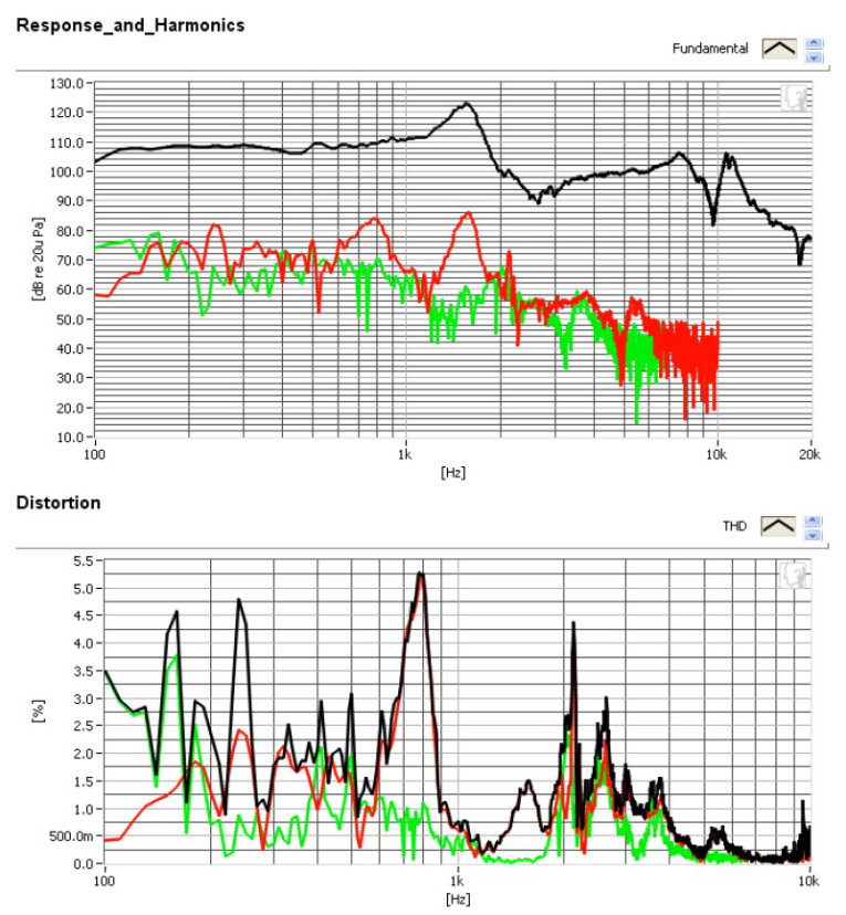
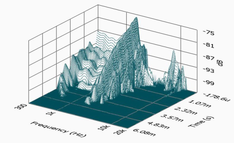
For the remaining series of tests, I used the Listen SoundCheck software, SoundConnect analyzer, and SCM microphone to measure distortion and generate time frequency plots. For the distortion measurement, I rigidly mounted the LW150-4 in free-air and used a noise stimulus to set the SPL to 94 dB at 1 m (7.85 V). Then, I measured the distortion with the Listen microphone placed 10 cm from the dust cap. This produced the distortion curves shown in Figure 13. I then used SoundCheck to get a 2.83 V/1 m impulse response and imported the data into Listen’s SoundMap Time/Frequency software. Figure 14 shows the resulting CSD waterfall plot. Figure 15 shows the Wigner-Ville (for its better low frequency performance) plot.
Overall, the LW150-4 delivers good performance from a 6” midbass driver, and especially one that is only 1.5” deep! For more information, visit www.daytonaudio.com. VC