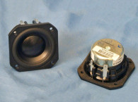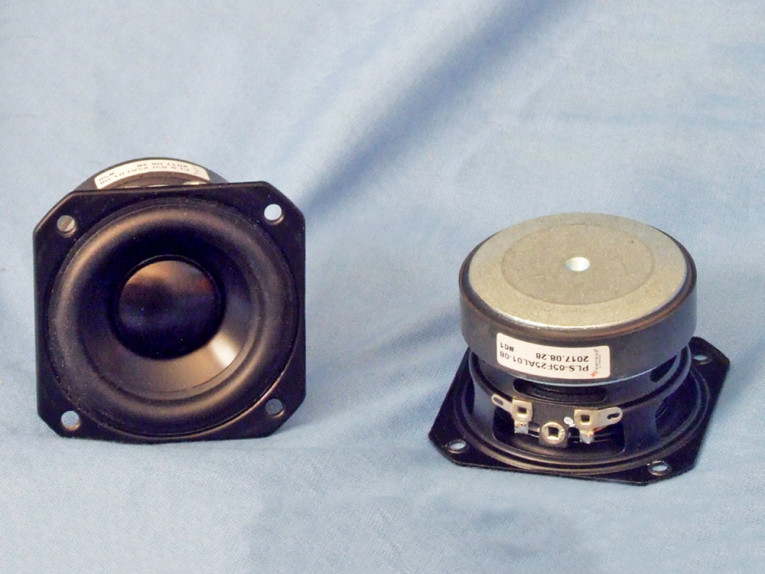
The cone assembly consists of a black anodized aluminum cone, with a 27 mm diameter aluminum dust cap (directly coupled to the voice coil former), and suspended with a NBR surround and a flat cloth spider (damper). Motive force for the cone assembly is supplied by a 60 mm diameter 14 mm thick ferrite motor that incorporates a copper cap shorting ring (Faraday shield) and a shaped T-yoke. Tinsel leads connect on one side of the cone to a pair of solderable terminals.
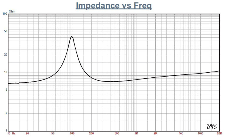
I commenced testing the PLS-65F full-range using the LinearX LMS analyzer and VIBox to create both voltage and admittance (current) curves, I clamped the driver to a rigid test fixture in free air at 0.3V, 1V, 3V, and 6V. It should also be noted that this multi-voltage parameter test procedure includes heating the voice coil between sweeps for progressively longer periods to simulate operating temperatures at that voltage level (raising the temperature to the first and second time constants).
Next, I post-processed the six 550-point stepped sine wave sweeps for each of the PLS-65F samples and divided the voltage curves by the current curves (admittance) to produce the impedance curves, phase generated by the LMS calculation method. I imported them, along with the accompanying voltage curves, into the LEAP 5 Enclosure Shop software. I selected the complete data set, the multiple voltage impedance curves for the LTD model, and the 1 V impedance curve for the TSL model in LEAP 5’s transducer derivation menu and created the parameters for the computer box simulations.
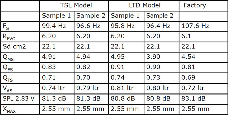
Figure 1 shows the 1 V free-air impedance curve. Table 1 compares the LEAP 5 LTD and TSL data and factory parameters for both of the PLS-65F samples. The LEAP TSL parameter calculation results for the PLS-65F were reasonably close to the factory data. As always, I followed my usual protocol and preceded to set up computer enclosure simulations using the LEAP LTD parameters for Sample 1. This consisted of a sealed box the same size as the ones used for the PLS-50N—a 61 in3 Butterworth sealed box with 50% fiberglass damping material and a 75 in3 damped Chebychev/Bessel vented alignment tuned to 74 Hz with 15% damping material in the box. Note that I used the simulated fiberglass (R19) selection in LEAP 5 primarily because it is accurate and a known commodity in terms of damping. However, due to its carcinogenic nature, fiberglass is almost never used anymore, although I have seen it in the past few years in the pro market. Most damping material used today is either foam or some form of Dacron batting. While LEAP does model polyester, the density is not as well established as fiberglass.

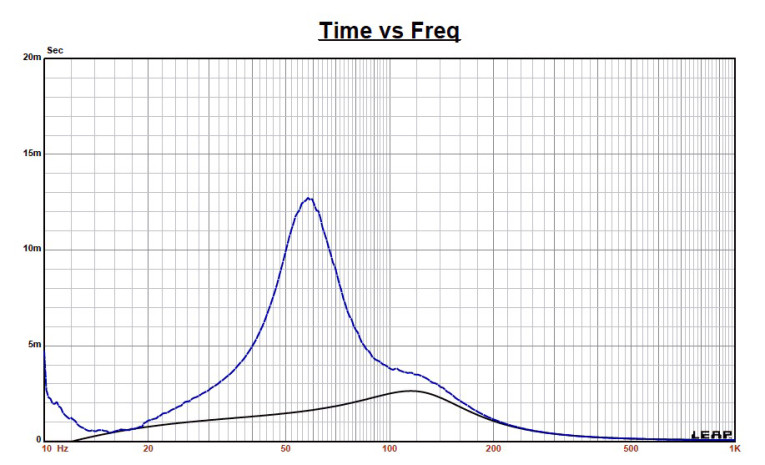
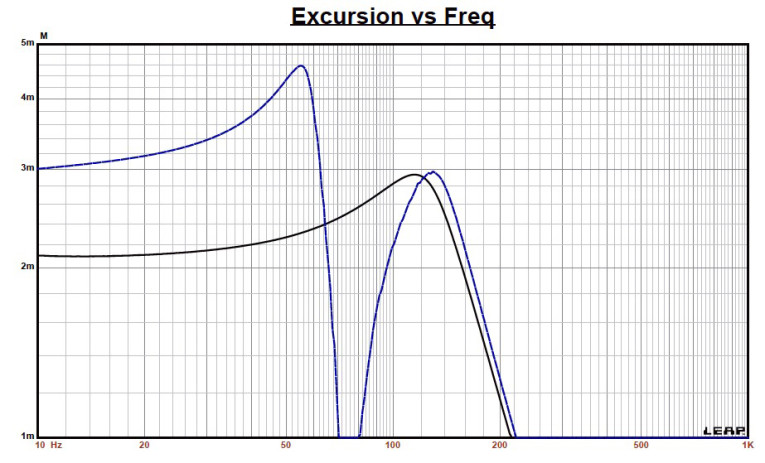
Figure 2 displays the results for the PLS-65F in the sealed and vented box simulations at 2.83 V and at a voltage level high enough to increase cone excursion to Xmax + 15% (2.93 mm for the PLS-65F). This produced a F3 frequency of 113 Hz (F6 = 94 Hz) for the 61 in3 sealed enclosure and –3 dB = 97 Hz (-6 dB = 67 Hz) for the 75 in3 damped Chebychev/Bessel vented simulation.
Increasing the voltage input to the simulations until the maximum linear cone excursion was reached resulted in 92.5 dB at 8.6 V for the sealed enclosure simulation and 96 dB with an 9.5 V input level for the vented enclosure. Figure 3 shows the 2.83 V group delay curves. Figure 4 shows 8.6 V/9.6 V excursion curves.

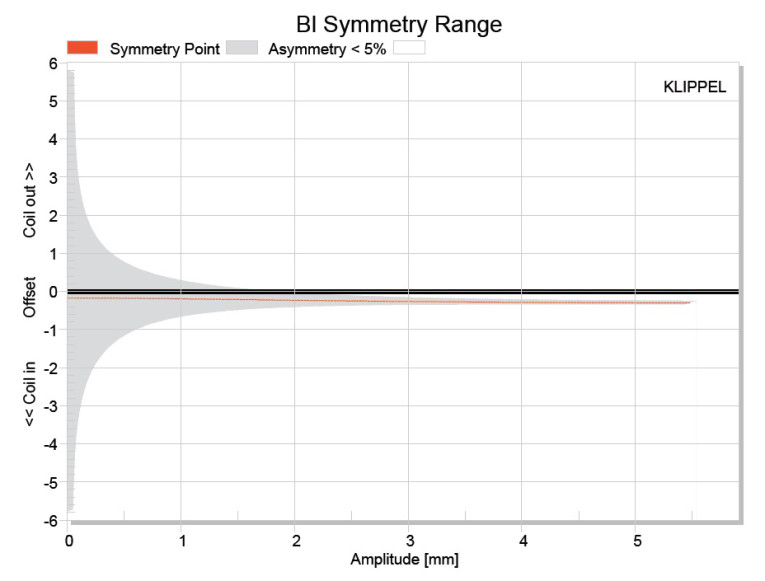
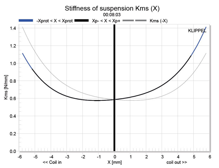
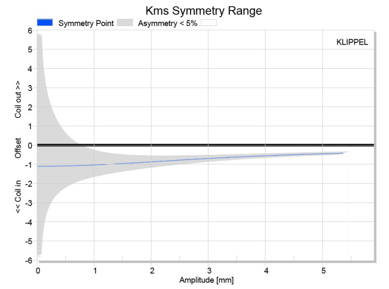
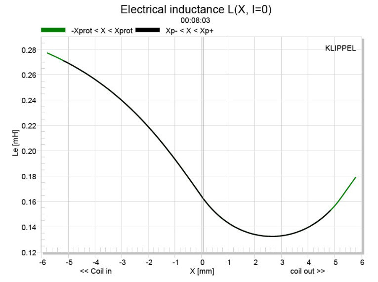
Figure 7 and Figure 8 show the Kms(X) and Kms symmetry range curves. The Kms(X) curve is moderately symmetrical and has a rearward (coil-in) offset at the rest position, and the physical Xmax position, which shows a high degree of certainty, is about 0.77 mm. Displacement limiting numbers calculated by the Klippel analyzer for the PLS-65F were XBl at 82% Bl is 2.3 mm and for XC at 75% Cms minimum was 3.3 mm, which means Bl is the most limiting factor for prescribed distortion level of 10%.
Figure 9 gives the inductance curve Le(X) for the PLS-65F25AL01-08. Inductance typically increases in the rear direction from the zero rest position as the voice coil covers more pole area. However, because this transducer has a copper cap shorting ring, the inductance variation is only 0.23 mH to 0.13 mH from the coil-in and coil-out Xmax positions, which is good.
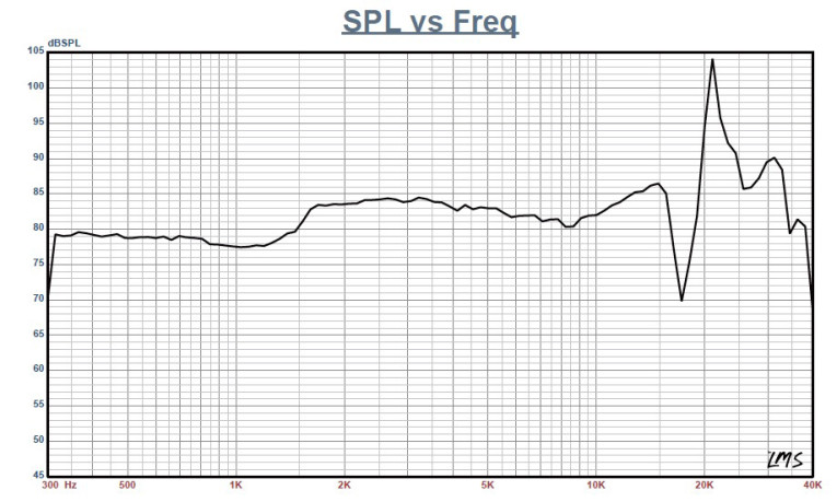

Next I mounted the PLS-65F in an enclosure, which had a 9” × 4” baffle and was filled with damping material (foam). Then, I used the Linear LMS analyzer, set to a 100-point gated sine wave sweep, to measure the transducer on- and off-axis from 300 Hz to 40 kHz frequency response at 2.83 V/1 m. Figure 10 gives the PLS-65F’s on-axis response indicating a smoothly rising response all the way out to 30 kHz, with an aluminum breakup mode at 21 kHz. There is a 6 dB shelf transition between 1 kHz to 2 kHz. Equalizing this to the level below 1 kHz would give a more balanced spectral profile, but at the expense at overall loudness.
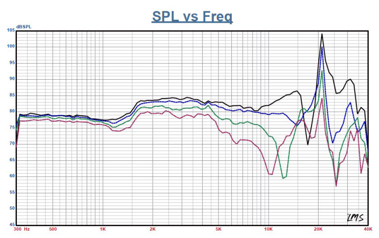
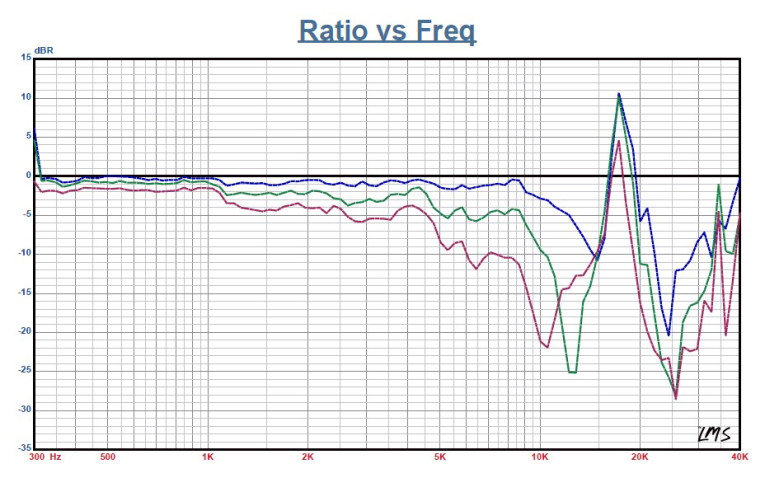
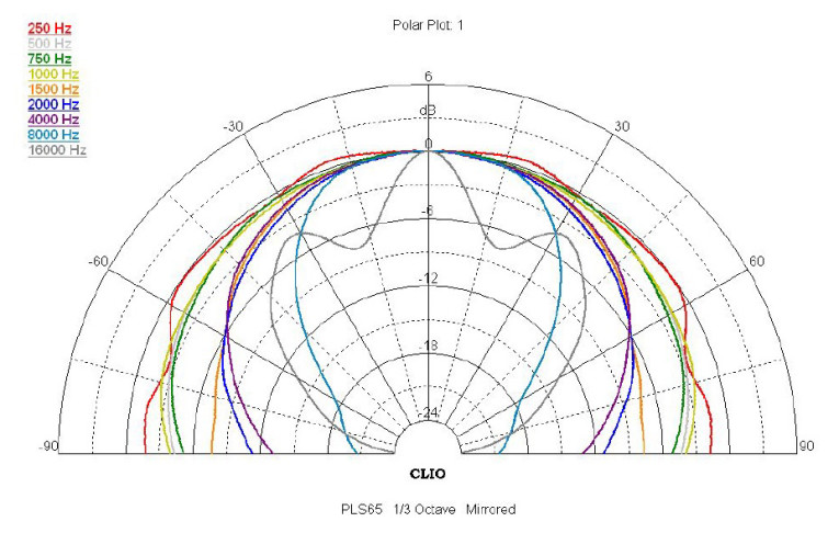
Figure 11 displays the on- and off-axis frequency response at 0°, 15°, 30°, and 45°. Figure 12 gives the off-axis curves normalized to the on-axis response. Figure 13 shows the CLIO 180° polar plot (measured in 10° increments). The two-sample SPL comparison is illustrated in Figure 14, indicating the two samples were closely matched within less than 1 dB out to 10 kHz.
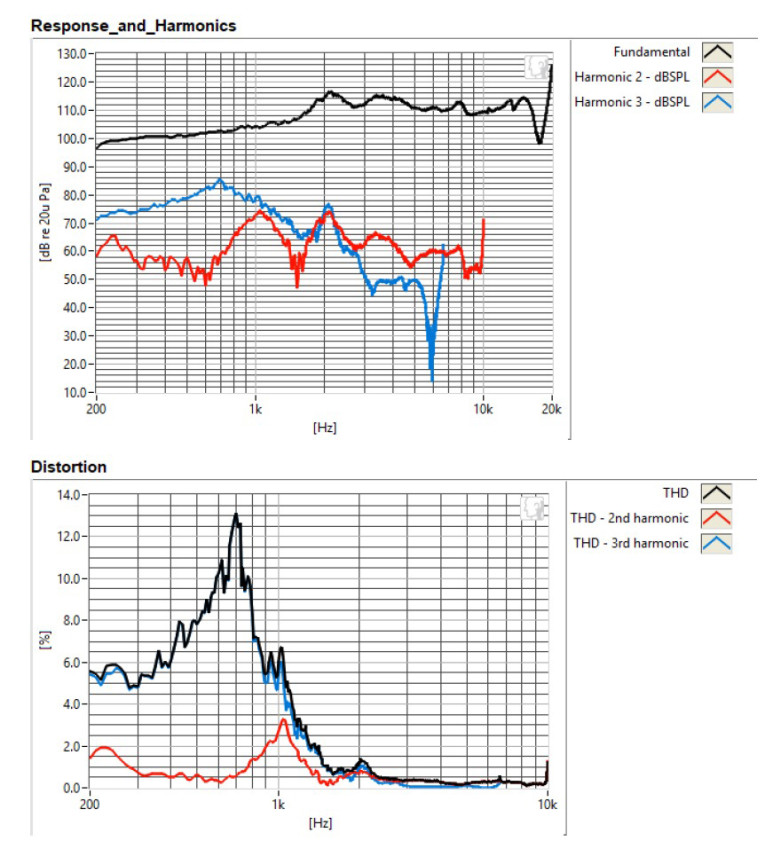
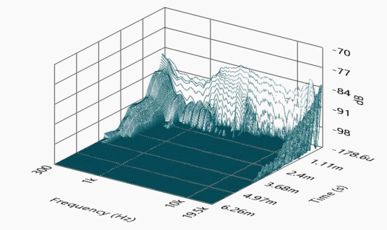
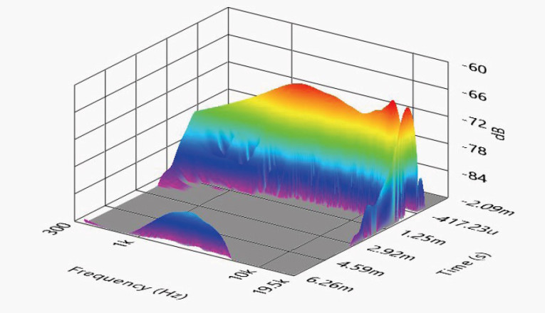
For the remaining series of tests, I employed the Listen AmpConnect analyzer operating with SoundCheck 15 along with the Listen 0.25” SCM microphone and power supply to measure distortion and generate time-frequency plots. For the distortion measurement, I mounted the Peerless woofer rigidly in free air, and used a noise stimulus to set the SPL to 94 dB at 1 m (7.3 V). Then, I measured the distortion with the microphone placed 10 cm from the dust cap. This produced the distortion curves shown in Figure 15. I then used SoundCheck to get a 2.83 V/1 m impulse response for this driver and imported the data into Listen’s SoundMap Time/Frequency software. Figure 16 shows the resulting CSD waterfall plot. Figure 17 shows the Wigner-Ville plot.
While the intended application for this Tymphany Peerless 2.5” full-range driver is TV, multimedia, lifestyle speakers, and the new generation of voice control smart speakers, Peerless does suggest that the device would also be good for pro sound line source applications. For more information about these well-crafted Peerless by Tymphany drivers, visit www.tymphany.com/peerless. VC
This article was originally published in Voice Coil, November 2017.