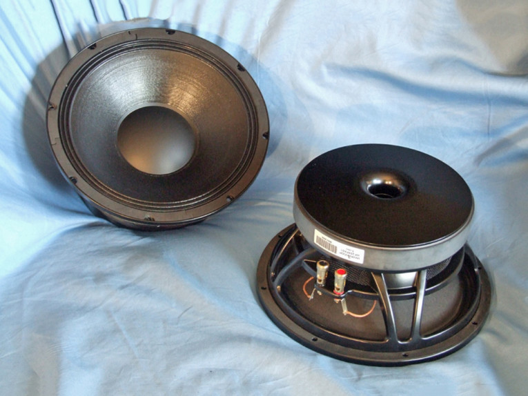

All this is driven by a 76 mm diameter (3”) voice coil wound with round wire on a vented black fiber glass non-conducting former. The motor structure powering the cone assembly utilizes a single 25 mm thick, 190 mm diameter ferrite magnet sandwiched between a black-plated 8 mm thick front plate and a black-plated and shaped T-yoke that has 30 mm diameter pole vent that is flared at both ends to suppress vent noise. As part of Wavecor’s Balanced Drive motor format, the WF259PA01 further incorporates an aluminum shorting ring (Faraday shield) that reduces distortion caused by eddy currents as well as a shaped extended pole piece. Last, the braided voice coil lead wires terminate to a pair of gold push button terminals.
I began characterizing the WF259PA01 using the LinearX LMS analyzer and VIBox to measure both voltage and admittance (current). Sweeps were generated in free air at 0.3V, 1V, 3V, 6V, 10V, 15V, 20V, and 30V. The measured Mmd that was provided by Wavecor (an actual physical cone assembly measurement with 50% of the surround and spider removed) was used rather than a single 1 V added (delta) mass measurement. It should also be noted that this multi-voltage parameter test procedure includes heating the voice coil between sweeps for progressively longer periods to simulate operating temperatures at that voltage level (raising the temperature to the first and second time constants).
I further processed the 16 sine wave sweeps for each woofer and divided the voltage curves by the current curves to produce impedance curves. I generated phase curves using the LEAP phase calculation routine, after which I copy/pasted the impedance magnitude and phase curves plus the associated voltage curves into the LEAP 5 Enclosure Shop software’s Guide Curve library. I then used this data to calculate parameters using the LEAP 5 LTD transducer model. Because most manufacturing data is produced using either a standard transducer model, or in many cases the LEAP 4 TSL model, I also generated LEAP 4 TSL model parameters using the 1 V free-air that can also be compared with the manufacturer’s data.
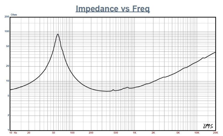
Figure 1 shows the 1 V free-air impedance plot. Table 1 compares the LEAP 5 LTD and LEAP 4 TSL Thiele-Small (T-S) parameter sets for the two Wavecor WF259PA01 driver samples along with the Wavecor factory data. From the comparative data shown in Table 1, you can see that all four parameter sets for the two samples were reasonably similar and correlated well with the factory data. As always, I followed my normal protocol for Test Bench testing and used the Sample 1 LEAP 5 LTD parameters and set up two computer enclosure simulations, one in a 0.75 ft3 QB3 vented enclosure with 15% fill material (fiberglass) tuned to 69 Hz and for the second example, a 1 ft3 Extended Bass Shelf (EBS) ported box also with 15% fill material and tuned to 60 Hz.
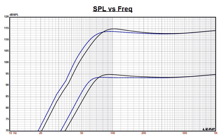
Figure 2 gives the results for the Wavecor WF259PA01 in the smaller and larger vented enclosures at 2.83 V and at a voltage level sufficiently high enough to increase cone excursion to Xmax + 15% (5.2 mm for WF259PA01). This resulted in a F3 of 67 Hz (-6 dB = 60 Hz) for the QB3 vented enclosure and a -3 dB for the larger vented simulation of 56 Hz (-6 dB =50 Hz).
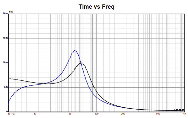
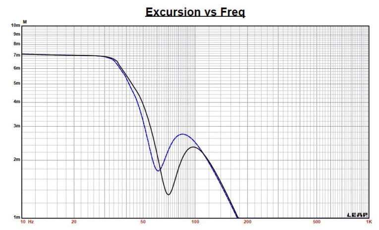

Increasing the voltage input to the simulations until the approximate Xmax + 15% maximum linear cone excursion point was reached resulted in 115 dB at 30 V for the smaller enclosure simulation and 114 dB with also at 30 V input level for the larger box. Figure 3 shows the 2.83 V group delay curves. Figure 4 shows the 30 V excursion curves.
Klippel analysis for the WF259PA01 produced the Klippel data graphs shown in Figures 5–8. (Our analyzer is provided courtesy of Klippel GmbH and the analysis was performed by Patrick Turnmire, Redrock Acoustics. Please note, if you do not own a Klippel analyzer and would like to generate this type of data on any transducer, visit www.redrockacoustics.com.)
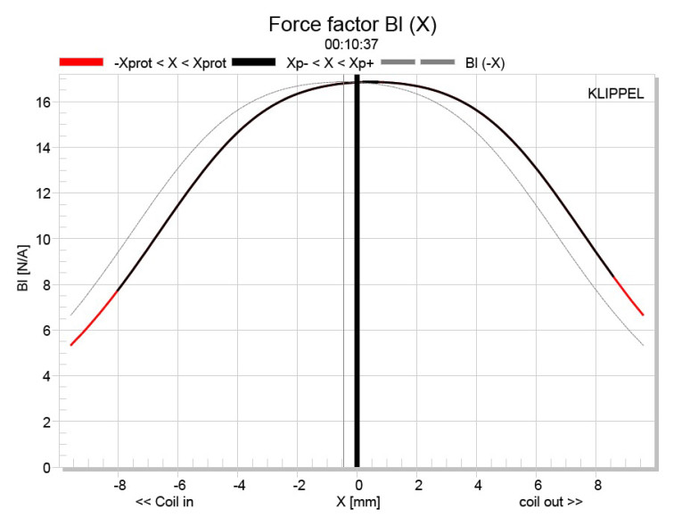
The Bl(X) curve for WF259PA01 seen in Figure 5 is moderately broad and mostly symmetrical, typical (with a small amount of offset) of a driver with a relatively high Xmax (4.5 mm is actually a generous amount of Xmax for the average pro sound 10”). Looking at the Bl symmetry curve in Figure 6 shows 0.48 mm Bl coil-out (forward) offset once you reach an area of reasonable certainty (3 mm), decreasing to 0.19 mm at the physical 4.5 mm Xmax position, and decreasing beyond that point, so a minor amount of offset.


Figure 7 and Figure 8 show the Kms(X) and Kms symmetry curves for the Wavecor subwoofer. The Kms stiffness of compliance curve seen in Figure 7 is also symmetrical, with but with more offset. The Kms symmetry range curve (see Figure 8) exhibits a minor 0.59 mm coil-out (forward) offset at a region of high certainty (1 mm) that increases to 0.68 mm by 4.5 mm Xmax position, which is still a minor amount of offset.
Displacement limiting numbers calculated by the Klippel analyzer, using the 10% distortion criteria for Bl, was XBl at 82% (Bl dropping to 82% of its maximum value) equal to 4.6 mm, just slightly above the Xmax number. For the compliance, XC at 75% Cms minimum was 3.3 mm, which means that for the WF259PA01, the compliance is the more limiting factor for getting to the 10% distortion level. Using the 20% distortion criteria, the numbers are both above Xmax with XBl = 5.8 mm and XC = 5.9 mm.
Figure 9 gives the inductance curve Le(X). Motor inductance will typically increase in the rear direction from the zero rest position as the voice coil covers more of pole, however, that doesn’t happen here. What we do get is lower inductance variation from full in to full out travel, which is the goal you want to achieve. The aluminum shorting ring is doing its job with inductance only varying less than 0.1 mH from -4.5 mm to +4.5 mm, which is reasonably minimal inductance change.

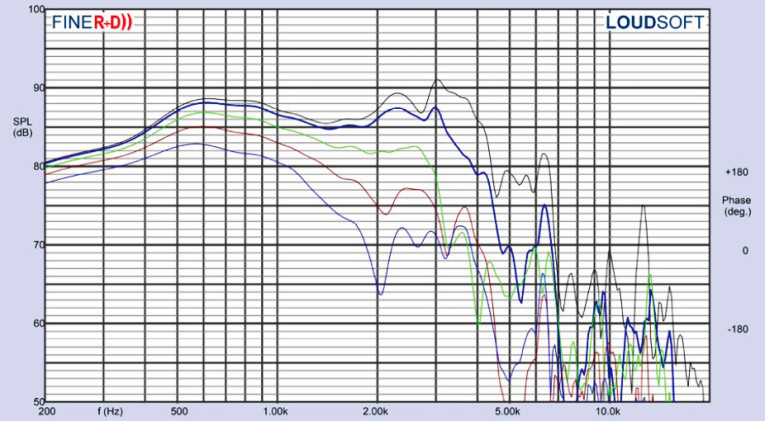


After the Klippel analysis, I mounted the driver in an enclosure filled with foam damping material and that had a 20” × 11” baffle area. I used the LOUDSOFT FINE R+D FFT analyzer to measure the WF259PA01’s SPL on and off axis. Figure 10 gives the on-axis response measured 200 Hz to 20 kHz at 2.83 V/1 m. The response is rising with no anomalies out to 2 kHz, with a breakup mode peaks up 5 dB at 2.2 kHz and 3 kHz just prior to the low-pass roll-off of the driver. Figure 11 shows the on and off axis to 60°, with the LMS generated normalized response shown in Figure 12, followed by the CLIO generated polar plot shown in Figure 13.
Finally, Figure 14 gives the two-sample SPL comparison showing, as you would expect from Wavecor, the drivers to be well matched to less than 1 dB throughout the relevant operating range up to 3 kHz.
Next, I used the Listen, Inc. AudioConnect analyzer to perform distortion and time domain analysis. Note that I recently swapped the Listen, Inc. SoundConnect analyzer with the built-in amplifier for the AudioConnect analyzer that allows for the use of higher watt outboard amplifiers (Thanks to Dan Knighten and Listen, Inc.!). For the distortion measurements, I set the voltage level with the driver rigidly mounted in free air and increased the voltage until it produced a 1 m SPL of 104 dB (6.8 V), which is my SPL standard for pro sound drivers. I made the distortion measurement with the microphone placed near-field about 10 cm from the dust cap. Figure 15 shows this graph, which actually includes two plots — the top graph being the standard fundamental SPL curve with the second and third harmonic curves and the bottom graph shows the second and third harmonic curves plus the THD curve with an appropriate X-axis scale.
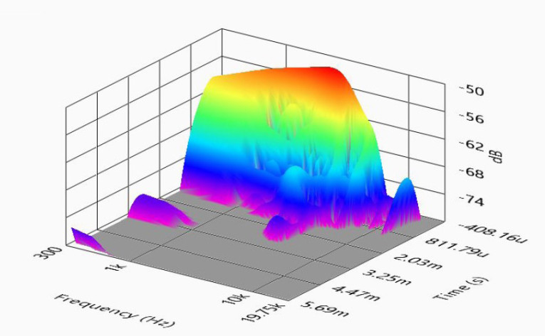
Interpreting the subjective value of conventional distortion curves is almost impossible; however, looking at the relationship between the second to third harmonic distortion curves is of value. I used SoundCheck 15 to get a 2.83 V/1 m impulse response (again with the driver mounted in the enclosure with the 20” × 11” baffle) and imported the data into Listen’s SoundMap Time/Frequency software. Figure 16 shows the resulting CSD waterfall plot. Figure 17 shows the Wigner-Ville plot (chosen for its better low-frequency performance).


I have used Wavecor drivers (both off the shelf and with proprietary modifications) on several projects as a consultant, and have a lot of respect for this China-based company. The F259PA01 10” pro sound woofer is another well-crafted transducer from the engineers at Wavecor, especially for its first foray into the pro sound market.
www.wavecor.com. VC
This article was originally published in Voice Coil, February 2018.