For those audio systems, the following measurements are recommended for quality assurance:
• Frequency response
• Phase response and polarity
• Harmonic distortion
• Sensitive Rub & Buzz for detection of loudspeaker defects
• Assembly faults (e.g., loose screws and parasitic vibrations)
• Air leakage detection (due to mounting or gluing faults)
• Ambient noise detection or immunity is recommended to avoid false rejects due to ambient noise.
Sophisticated signal processing algorithms need to be fed with relevant response data from the device under test (DUT). Due to significant delays, feeding correct data is quite challenging when using external signal sources. This article discusses methods for coping with unknown, varying, or even unpredictable delays in the measurement chain while still fulfilling all requirements for quality assurance applications.

The Analysis Window
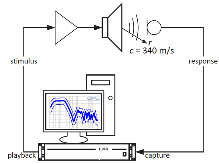
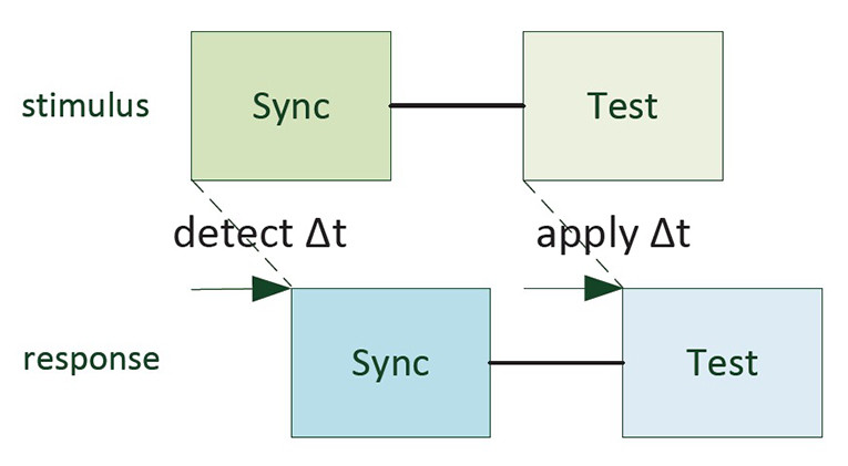
The analysis window describes the time window where response data is recorded and fed to the analysis algorithms. It usually has the length of the stimulus. Any audio measurement system needs to obtain the response of a DUT. In standard measurement situations, the stimulus is played back without a delay and the capture process is synchronized to the playback (see Figure 1). Thus, the temporal position of the response data is known and the analysis window is optimally placed automatically.
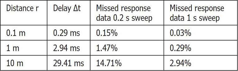
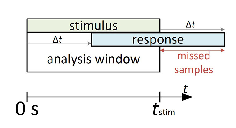
When one measurement device is used, playback and capture processes are sample-synchronous and the internal delay is compensated automatically. In that case, the response is usually only delayed due to distance of acoustical source and microphone. The acoustical delay causes a slight shift of response data in the analysis window (see Figure 2). The shift causes the last part of the response to be outside of the analysis window. As the delay is usually very small, the number of missed samples is negligible compared to the complete response (see Table 1).
For a single sweep, the relevance of the missed response samples depends on the actual delay Δt and the length of the analysis window. For measurement setups with up to 1 m distance between the source and the microphone, the impact is small for a 1s sweep. For ultra-fast stimuli, distances above 1m should be avoided.
What if delays are not negligible? In some measurement setups, the distance between acoustical source and microphone is not the only reason for a delay. Other factors may introduce significant additional delays including:
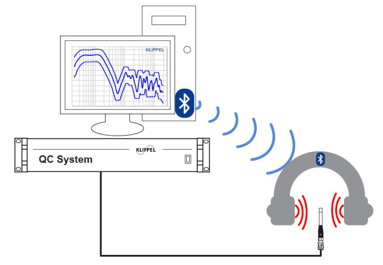
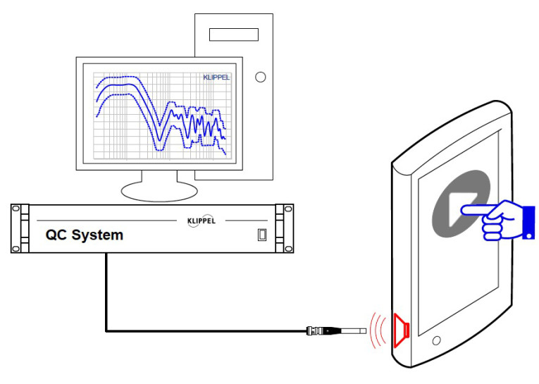
• Usage of third-party audio devices for playback and/or capture processes instead of a measurement instrument (see Figure 3):
• Drivers and the operation system’s audio architecture will introduce latencies. Due to the dynamic definition of the driver’s buffer sizes, those delays will be different on every driver initialization (see Figure 4).
• Sample drift of audio devices: Using mixed configurations (different audio devices for playback and capture) without synchronizing sampling clocks will cause a drifting delay vs. time.
• Other delays in the signal chain: If digital signal processors and wireless technologies are included in the measurement, additional delays will be introduced.
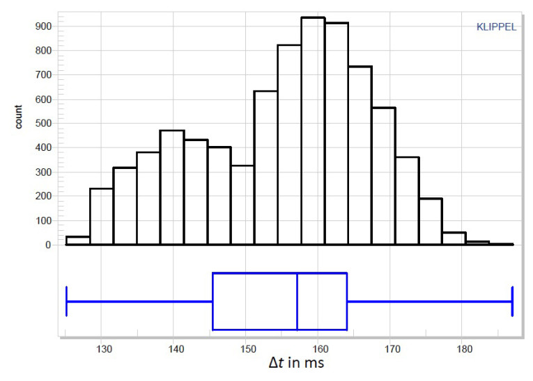
Those delays are usually constant. Figure 4 shows the delay distribution of 7,800 measurements using a mixed configuration (e.g., playback with Bluetooth audio, capture with Klippel QC hardware). The audio devices were re-initialized before every measurement. The mean delay of around 155 ms varies by approximately ±35 ms. (That would correspond to an acoustic delay due to a varying distance of ±12 m.)
The delay and its variation cannot be neglected. Otherwise a tremendous amount of data is lost. See Figure 5 for the analysis yielding measurement results with questionable relevance. What if the moment of playback is completely unknown? With some measurement setups, the moment of playback (and thus, the moment of time when the response hits the microphone) is completely unknown. This is the case if playback and/or capture processes are completely autonomous and not synchronized.
An example is the manual trigger of playback of a sound file on a tablet device (see Figure 6). Other examples are complex audio systems, where the playback is triggered by automation processes (e.g., in-situ quality control in automobiles at the end of the assembly line) or mobile measurements (e.g., checking the loudspeakers of an alarm system in an airport with a handheld recorder and post-processing the response data).
These wave file-based measurement setups have to be used if the audio system under test does not provide a suitable signal input/output. The problem of placing the analysis window in the correct moment of time is similar to the mixed configuration setup, but with unpredictable delay between measurement start and actual playback.
Solving the Problem
Measurement systems that cope with unknown/varying or even unpredictable delays often use one of the following solutions:
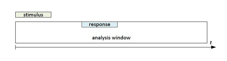
• Increase the length of Analysis Window — By using a longer analysis window, the need to perfectly position the initial analysis window is relaxed, assuming that the complete response is captured somewhere in the large analysis window (see Figure 7). Subsequent algorithms (e.g., the calculation of impulse response) may place a refined analysis window of shorter length at a more precise moment of time. A major drawback of this method is the time consumed. It is not suitable for automatic wave file-based measurements since the assumption that the complete response was captured might not be true. Moreover, this method does not address the problem of sample drift. Even if the complete response was captured, it might not be detectable in the impulse response for fine-tuning due to sample rate deviation.
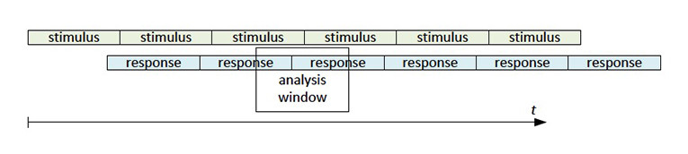
• Looping the stimulus — Looping the playback of the stimulus may eliminate the need to position the analysis window at all (see Figure 8). This is applicable for all steady-state signals (e.g., sinusoidal tone, multitones, or noise signals) or even a repeated sine sweep. The analysis window is arbitrarily placed in the response stream. If necessary, the response data may be mapped circularly to yield a corrected response block. This method is very time-consuming and adds the demand of repeatability to the stimulus. Furthermore, a significant amount of energy is put into the system. If a repeated sweep is used, room acoustics might falsify results (e.g., THD) or even mask defect symptoms.
• Trigger the measurement system — Triggering the measurement system at the correct point of time is the most time-efficient method to position the analysis window. The conventional method uses a sinusoidal energy trigger. This tone is detected in the recorded data stream and as soon as it is recognized, the measurement system starts capturing. The detection of a tone is time-consuming, inflexible, and relies on a very narrow frequency band. A sample accurate delay estimation can not often be achieved. Correlation techniques could also be used to detect the starting point of the response data. Complex stimuli could be used, which provides a more robust method.
Usually these methods do not address a possible sample rate deviation between capture and playback devices. Eventually, they will fail when the deviation or the stimulus length grows.

New Synchronization Method
The new synchronization method uses either an additional broad-band signal (pink or white noise) or the stimulus itself. By using an additional trigger signal (see Figure 9), a unique ID (e.g., a fingerprint) is injected in the noise signal. Only this specific ID will be able to successfully synchronize and trigger the system.
Thus, the synchronization signal for each test type is unique, which ensures using the correct response for a measurement. An additional noise signal should be used if long test stimuli are used for a measurement (above 2 s). By having the stimulus directly as the trigger (see Figure 10), the consumed overall time is kept small because no additional signal needs to be introduced in the sequence. All synchronization signals provide a sample rate tolerance of up to ±10 % for the synchronization process. That means a sync response is also detectable if the stimulus is mistakenly played back with 44,100 Hz sampling frequency instead of 48,000 Hz. To meet all measurement situations, two basic time regimes are provided:
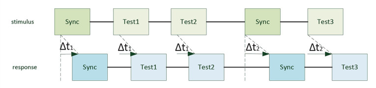
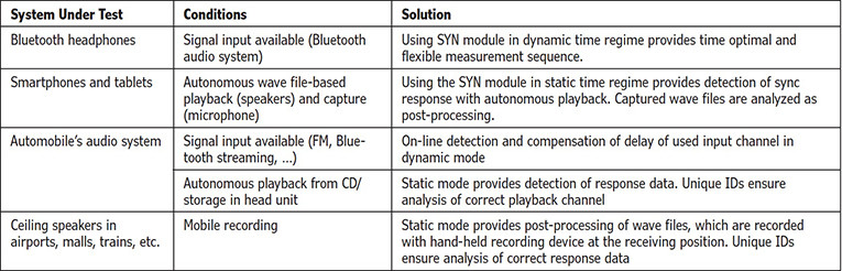
1. A dynamic time regime (see Figure 11) detects and compensates delays online. This mode can be used if the playback and capture streams are under control of the measurement system. A sync response is detected sample-accurate. Subsequent measurements are analyzed with an optimally positioned analysis window. A synchronization signal is played back before the test signals. Optionally, a re-synchronization within the sequence may be used to compensate for drifts of sample rates between capture and playback streams.
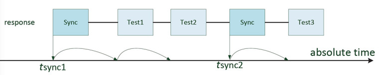
2. The static time regime (see Figure 12) handles measurement setups with completely autonomous playback (or capture) processes (e.g., wave file-based measurements). Here, the absolute durations and gaps between all signals are fixed. Again, a synchronization is requested at the beginning of the sequence to provide optimal placement for the analysis windows of subsequent measurements (now based on an absolute time axis). Optional resynchronization may compensate for sample rate drifts. With the static time regime, it is possible for standard sequences to be reused in several applications (like a standard audio test CD).

The synchronization search is based on overlapping block-wise analysis (see Figure 13). The evaluation is based on the calculation of the impulse response. If a valid impulse response is found, the synchronization is successful. Based on the position of the main impulse in the window, the delay (dynamic time regime), or the absolute position (static time regime) is determined. The temporal position of subsequent response data is calculated based on the delay or the absolute position of the synchronization.
When a significant sample rate deviation is present, this technique would fail if used solely. The new method is able to find the synchronization by reconstructing the original time axis before the calculation of the impulse response. Multiple paths of sound distribution (and multiple peaks in the impulse response) are handled by a smart look-ahead algorithm making sure that the incident of direct sound is used for synchronization.
This new synchronization technique is available as an add-on for the Klippel QC system as the External Synchronization (SYN) module. It ensures reliable and efficient synchronization of playback and capture while allowing use of the Klippel QC system.
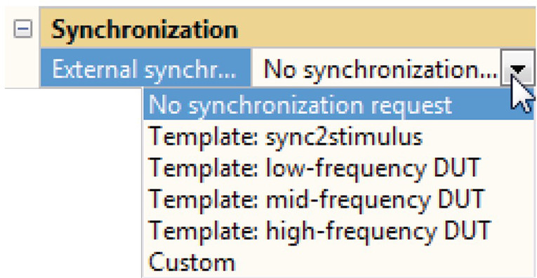
The SYN module setup is fairly easy. All the features run in the background and do not require user configuration (see Table 2). The user defines a synchronization request by selecting the channel characteristics from a set of templates (see Figure 14). A custom mode provides options for fine-tuning in special cases.
In Summary
In measurement situations with unknown, varying, or unpredictable delay between playback and capture processes, the analysis window needs to be aligned to the response data. This synchronization process is required to be robust, fast and universal. Klippel’s SYN module provides an advanced synchronization technique with simple setup integrated smoothly in the QC system. Even for complex test situations an exact synchronization, optimal placement of analysis windows and accurate measurements can be ensured.
www.klippel.de. VC
This article was originally published in Voice Coil, January 2017.