I have heard the following question asked many times: “How do I align a subwoofer with a full-range loudspeaker system?” I thought it might be interesting to delve into this to see if I could come up with an answer. The task of adding a subwoofer to a loudspeaker system to increase the low-frequency bandwidth should typically entail three primary items:
• The relative bandwidth of the subwoofer and the full-range system (crossover)
• The relative output level of the subwoofer and the full-range system (gain)
• The relative arrival time of the signal from the subwoofer and the full-range system (delay)
It is this last item that is perhaps the most challenging. This is the one that we will primarily investigate. We will also look at the first item briefly. With these taken care of, the second item should not be too much of a problem.
Loudspeakers, by their nature, are band-pass devices. To simplify the measurements and make it easier to see what’s going on with the graphs, I will use high-pass and low-pass filters instead of actual loudspeakers. The results will be the same with one exception: microphone location. Since our examples don’t use a microphone (only electrical measurements), it can’t be moved to a different location. This can be much more critical for measurements at higher frequencies because the directivity response of a loudspeaker will lead to differences in the measured response of a device at different locations. For devices that are, for the most part, omni-directional in the lower-frequency region, this will not be an issue.
There is another issue, of which one should be aware, concerning microphone placement that could lead to measured differences. That is the potential change in path length from the two devices under test (lower-frequency device and higher-frequency device) to the measurement microphone (or the listener’s ear.) At one mic position there may be very good summation. At another location, where the path length difference has changed by one-half wavelength of frequencies in the crossover region, there will be a notch (cancellation) in the summed response. When making field measurements, it is advisable to place the microphone(s) in position(s) that are typical of magnitude and arrival time differences to which most of the intended coverage area will be subjected.
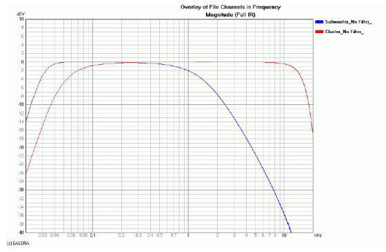
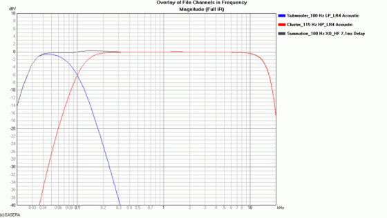
Let’s imagine a hypothetical system that has a full-range cluster that reproduces 60 Hz to 14 kHz adequately. We will add a subwoofer that is physically displaced from the fullrange cluster. The subwoofer reproduces adequately down to 30 Hz. These response curves are shown in Figure 1. We want a crossover at 100 Hz with a 4th order Linkwitz-Riley alignment.
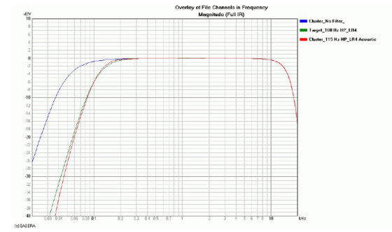
We can simply apply a 4th Linkwitz-Riley low-pass filter at 100 Hz to the subwoofer since its response is relatively flat, well above the intended crossover region. This is not the case for the cluster, however. Its output is already beginning to decrease, with decreasing frequency through the intended crossover region. We will need to apply an electrical filter that, when combined with the natural response of the cluster, will yield an acoustical output that matches a 4th order Linkwitz-Riley filter with an Fc of 100 Hz. Figure 2 shows the natural output of the cluster and the target Linkwitz-Riley response along with the cluster’s output after it has been high-pass filtered. A 3rd order Butterworth high pass at 115 Hz was used to get this response. A lower Fc and a parametric EQ filter might be used to achieve a more exact match. The response shown will be close enough for our purposes.
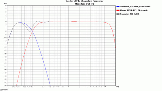
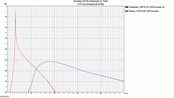
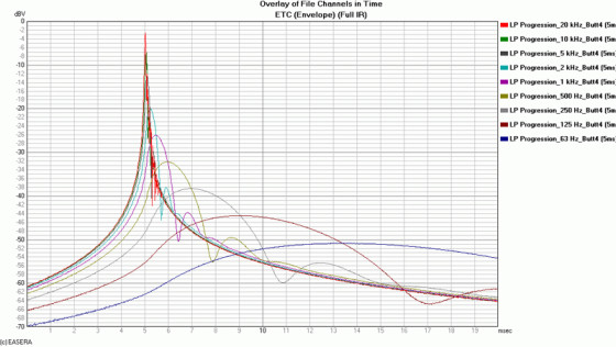
When the outputs of the two devices are combined, we get the responses shown in Figure 3. The summed magnitude response is not at all what we want. It is clear that something is causing cancellation. We know that the acoustic Linkwitz-Riley response of each device should sum to a flat response. Since it doesn’t, this would seem to indicate the problem is a misalignment of the two devices in the time domain. Looking at the Envelope Time Curve (ETC) of the passbands (see Figure 4) confirms that they are not synchronized.
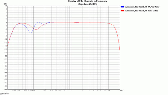
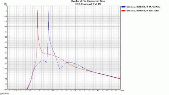
We need to delay the cluster, but by how much? If we choose to align the cluster’s peak arrival with the peak arrival from the subwoofer, we need to delay the cluster 14.7 ms. Alternatively we might choose to try to place the arrival of the cluster more towards the leading edge of the subwoofer’s ETC. This will require approximate 10 ms of delay for the cluster. The frequency and time domain of both these scenarios are shown in Figure 5 and Figure 6. Neither of the frequency domain curves looks like what one would consider good summation (reasonably flat response). The time domain would seem to indicate that the shorter delay is closer to the ideal response than the longer delay. We could go on guessing at different delay times in an attempt to optimize the response in both domains. Hopefully, there is a better way.
The underlying problem is that we have only low-frequency information output from the subwoofer. From the equation:
Δt =1/ Δf
where Δt is time resolution and Δf is frequency resolution, we can see that high-frequency resolution (small value of Δf) will yield low-time resolution (large values of Δt). We need higher-frequency output from the subwoofer (corresponding to higher Δf, lower-frequency resolution) to increase the time resolution in order for us to know when to position the cluster. If possible, we can bypass the low-pass filter on the subwoofer to get more high-frequency content in the output signal. This may help in more precisely determining the arrival time of energy from the subwoofer. Let’s assume that we can’t do this or if we can that it still doesn’t give us sufficient time resolution.
What we need is a way to get precise time information without high-frequency content. This is a seemingly impossible task, but only so in the time domain. In the frequency domain, there is a metric available that yields quite precise relative timing information. This is the group delay. The group delay is defined mathematically as the negative rate of change of the phase response with respect to frequency.
τg = −dφ / dω
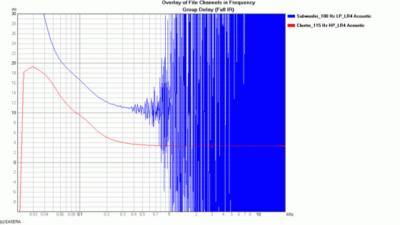
Figure 3 and Figure 4 show different views (domains) of the same measurement for the individual passbands. If we look at the group delay of this same data, we can derive some valuable information. The high-frequency limit (plateau) of each curve indicates the arrival time of the signal from that device. From this we see that the cluster arrival time is approximately 3.3 ms. This correlates very well with the ETC in Figure 4.
Don’t let the appearance of the subwoofer curve in the high-frequency region be bothersome. This is due to the low signal-to-noise ratio of the measurement above 400 Hz.
Referring to Figure 3, the output of the subwoofer is less than –24 dB at 200 Hz. Our use of a 4th order filter would indicate a level of less than –48 dB at 400 Hz and decreasing rapidly. It’s no wonder there is an SNR problem at higher frequencies.
We can look at the subwoofer curve around 300 Hz to get an indication of the high-frequency limit of its group delay. This turns out to be approximately 11.0 ms. The group delay of the cluster at this frequency is approximately 3.9 ms. This is a bit different than the 3.3 ms at higher frequencies.
This is caused by the phase shift of the high-pass filter and the natural high-pass response of the device. The low-pass filter being used on the subwoofer will have similar phase shift, and consequently, similar group delay differences in the high-frequency region if our measurement SNR was good enough to see it.
Taking the difference in 11.0 ms and 3.9 ms we now have a value of 7.1 ms to use as our delay setting for the cluster. This yields the summation, along with the individual passbands, shown in Figure 8 and Figure 9. This is almost the exact response we desire. There is less than 0.5 dB error in the vicinity of 150 Hz. This error is due to the output of the cluster and high-pass filter not exactly matching the Linkwitz-Riley target (see Figure 2).
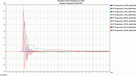
There is one more item that I think might be of interest in helping to see how a low-pass filter response affects apparent arrival time. I say apparent because it only appears that the arrival time is changing. Figure 10 and Figure 11 show the ETC and IR, respectively, of a 4th order Butterworth low-pass filter. The only difference in these curves is the corner frequency (–3 dB point) of the filter. The true arrival time for all of these filter curves is 5 ms. A complementary high-pass filter with an arrival time of 5 ms will combine properly with its lowpass counterpart in the graph. If the high pass is delayed so as to place the arrival so that it occurs later than 5 ms, there will be errors in the summation of the filters just as was illustrated in Figure 5 and Figure 6.
We have seen how the response of an electrical filter can combine with the response of a loudspeaker to yield the desired response (alignment) from the combined output. We have seen how the low-pass behavior of a device may make it appear that its arrival time is later than it actually is. We also demonstrated how to use group delay to determine the correct delay setting with relatively high precision when the high-frequency output of a device is limited due to its low pass behavior. I hope that some will find use for these techniques.

Charlie Hughes earned a physics degree from the Georgia Institute of Technology in1988. After graduation he worked for Peavey Electronics in Meridian, MS as a loudspeaker design engineer where he remained for 14 years. In late 2004, he started his own company, Excelsior Audio, located near Charlotte, NC. Excelsior Audio primarily provides consultation, design, measurement, loudspeaker optimization, and related services to loudspeaker manufacturers. More about Charlie Hughes