So, what if our listening room (or space) does not conform to this simplification? Well, if this is your problem or your area of interest, you will find something here for you.
A Simple Setup
The simplest configuration of a subwoofer system consists of a single subwoofer and two wide-range loudspeakers. The subwoofer is typically positioned in the “widely recommended” corner location, and the two wide-range loudspeakers are placed to produce an acoustic stage image for the listener. “Which corner?” you may ask. Well, not all corners are equal, as you will see. In my previous articles on loudspeaker placement (See References 3,4,5,6), I emphasized the importance of understanding the location of the room’s nodal lines and pressure maximum. Now I extend the analysis and actually generate the “room contribution” curves for a non-rectangular
room.
Here, I am talking about SPL of an “ideal” speaker with a flat frequency response from 0–200Hz. Two such subwoofers are placed in the room, and the resulting SPL is plotted up to 200Hz. Showing only the room contributions offers better clarity for visualizing the room modal response, because it is not obscured by the subwoofers’ own irregular SPL.
The Basics You Know
As you know, all rooms (a cavity volume enclosed by walls) have resonant frequencies at which the SPL generated by a source can be quite large. The frequencies at which resonances occur (called modes) depend on the geometry of the room. At a resonance frequency the pressure pattern inside the room will consist of antinodes, where the pressure is maximum, and nodes, where the pressure is zero. In a room with hard (e.g., reflective) walls, the pressure will always be maximum at the wall or in a corner when the room is excited at any of its modal frequencies.
If the source is located at an antinode for a given mode, the room response will be greatest. If the source is located at a pressure node for a given mode, the room will not respond regardless of how powerful the source is. Some of us (myself included) take advantage of our listening room’s acoustic behavior to improve the performance of our systems. Placing a loudspeaker or subwoofer against a wall or in the corner of a room allows the low-frequency modes of the room to enhance the low-frequency performance of the loudspeakers.
When you place the source at a node for that frequency standing-wave pattern, the maximum room response drops to zero at that frequency. Moving the speaker some distance away from the node restores (at least partially) the room’s response. Modal patterns occur only when the room is being driven at a modal frequency. At any other frequency, the pressure waves radiating outwards from the source reflect from the walls, but do not combine to produce a modal pressure pattern. As a result, there are no nodes and antinodes and the pressure can actually fall to zero at a wall.
A Leap Beyond the Rectangular Room
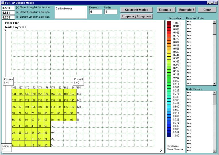
If I were to model a low-frequency loudspeaker generating pressure patterns in a simple, six-wall room, I could simply employ a closed form equation based on the summation of images. However, in a more general case, the room will not be a simple six-wall cavity6. In that case, I would resort to the Finite Element Method (FEM) to take advantage of its accuracy at low frequencies and its excellent handling of complex geometrical shapes (7). Figure 1 shows a floor plan of an “L-shaped” room with subwoofer 1 (Sw1), subwoofer 2 (Sw2), and listener (L1) located at nodes “186,” “188,” and “0,” respectively.
I have also used “brick” elements to approximate my listening room’s internal geometry for the purpose of producing the FEM mesh. The “brick” element has the following dimensions: X = 0.50m, Y = 0.611cm, and Z = 0.25cm. With these dimensions in mind, I will get 20 elements per 20Hz acoustic wave and only two elements to approximate 200Hz wave.
It is obvious that the accuracy of my model deteriorates as the frequency increases. I could have chosen smaller elements and readily improved the accuracy at 200Hz. This would be great, but the penalty would be increased calculation time and RAM usage. It is probably worth mentioning that although my analysis covers the frequency range up to 200Hz, I am mostly interested in frequencies below 100Hz. These are easier to discriminate from the SPL modal plots and have more defined pressure patterns. Additionally, the low-end modes are more widely spaced, and therefore easier to deal with without affecting the immediately adjacent modes.
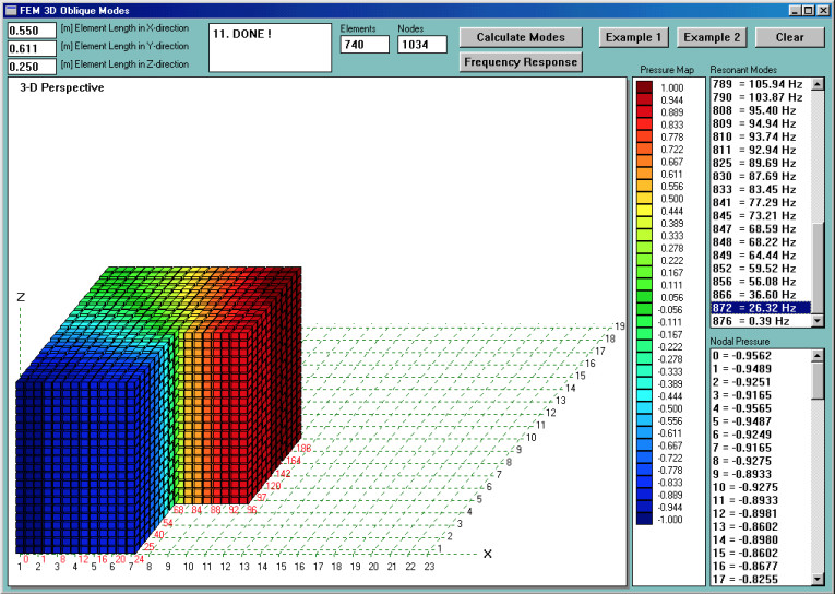
As a starting point, I have determined room modes. Some of the results are shown in Figs. 2–5. You can easily observe that, generally, modal (minimum pressure, deep green color) lines are not straight. They curve within the room and their locations are not immediately obvious without the FEM analysis. As I mentioned before, knowing your room nodal lines will help you determine where not to place your subwoofers.
Modal analysis revealed that the lowest modes are: F1 = 27Hz, F2 = 36Hz, F3 = 54Hz, F4 = 57Hz, F5 = 64Hz, and F6 = 73Hz. There are many more modes below 100Hz, but for the sake of clarity, I will focus only on those I mentioned. It is easy to observe that areas of maximum pressure (antinodes — deep red color for positive pressure or deep blue color for negative pressure) are always located near the walls or corners.
According to what I have just said, you would be tempted to locate your single subwoofer in one of those corners to take maximum advantage of the “room gain” effect. You may have also convinced yourself that you should place your subwoofer this way to allow the speaker to excite the maximum number of room modes, and preferably all room modes. This way, the smoothest (although still quite irregular) overall frequency response could be achieved. Here the “golden ratios” of room dimensions come into focus. The idea is to position room modes evenly across the low-end frequency range, which you can do by affecting room geometry.


Modal Analysis
Anyway, armed with all this common knowledge, I continue looking at Fig. 2, which, at first, you may find quite contradictory to what I just said. Why? Well, I have just said that pressure maximums are located at the room’s corners. But, in Fig. 2 you’ll note corner “A,” with the 26.32Hz nodal line (minimum pressure) sitting right at it. This is exactly the opposite of my previous statement ...or is it?
Before I go any farther, let me point out the advantage of FEM employed for this analysis. Of course FEM is complex, but it allows you to see and model things that would not be readily possible without it. Now, back to solving the problem.
The answer lies in the room’s “Lshaped” geometry. The corner “A” is located almost exactly halfway between corners “B” and “C.” As you can see in Fig. 2, the 26.32Hz mode would develop between those two corners, so the pressure maximum would be located in those corners. It should be easy to envisage that the nodal line for this particular mode should fall right in the middle between these two corners. If you could “unfold” the room, (imagine corners “C,” “A,” and “B” lined up), you would find corner “A” sitting in the middle of the long wall marked by corners “C” and “B.”
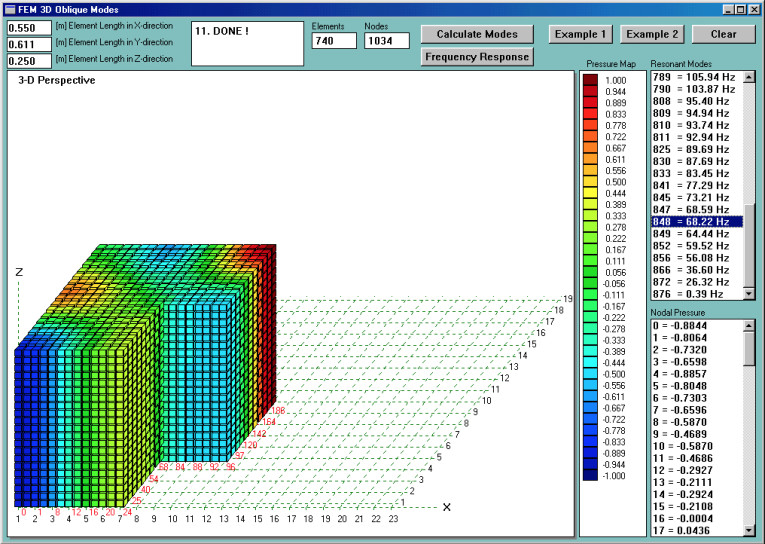
The problem actually becomes worse. If you examine Fig. 5, you will find the same issue at 68.22Hz. This is not exactly the harmonic of the 26.32Hz mode because the room has shorter walls on one side than the other. Once again, corner “A” has a nodal line right across it. You may expect this to happen at higher frequencies as well. I hope this short explanation of Fig. 2 and Fig. 5 offers you some indication of the importance of modal analysis, because it offers significant insight into the physics of your room acoustics.
Analysis Of Room Contribution
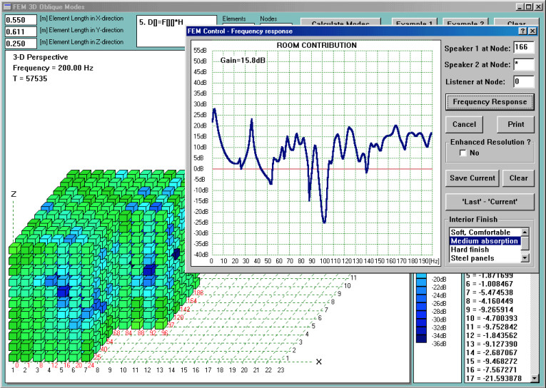
As a test case, I decided to place my subwoofers as described in Fig. 1. Now, having performed the modal analysis, I anticipate that there will be differences between subwoofer 1 and subwoofer 2 SPL plots. First, I need a reference “room contribution” coming from both subwoofers.
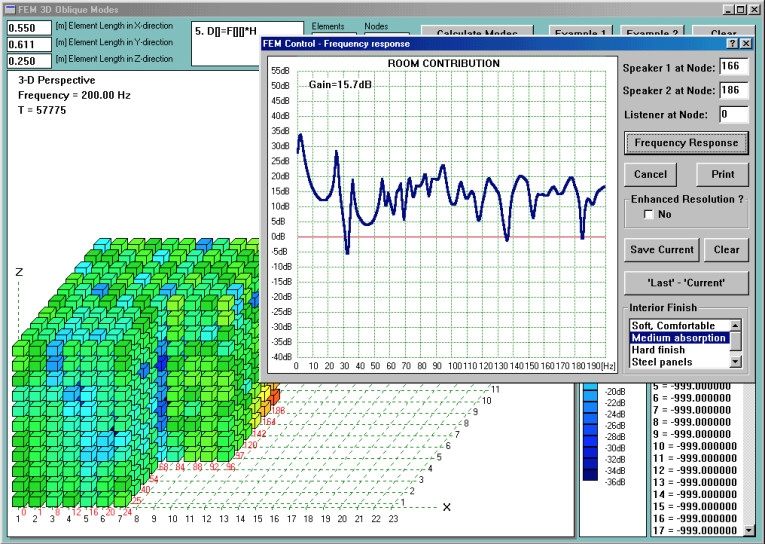
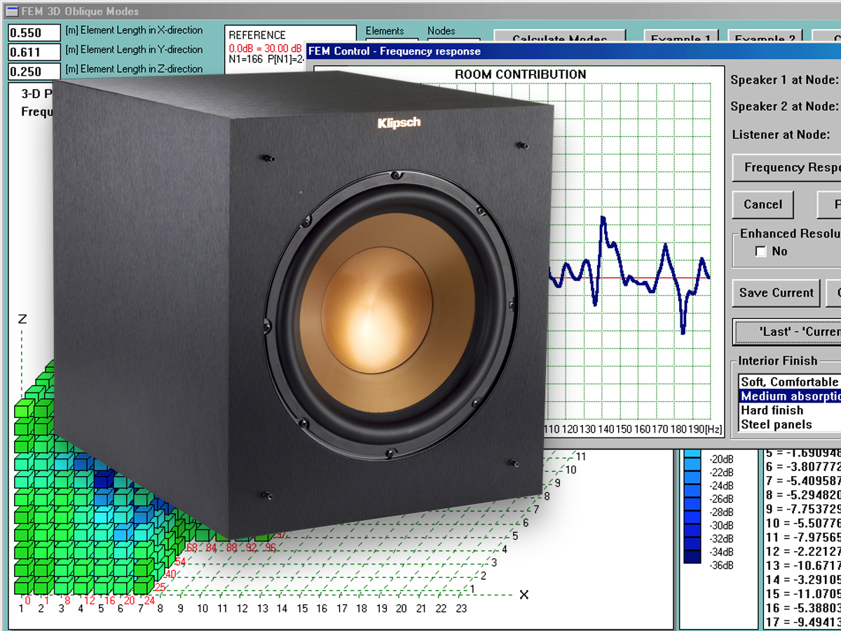
This reference plot is shown in Fig. 6. As I discussed before, there will be frequencies, where there are pressure minimums at the listener location at the wall. The most evident are 32Hz, 136Hz, and 184Hz, where the outward radiating pressure waves combined destructively and produced a node at the listener 1 location. The “notches” due to this are fortunately quite narrow. You may notice that the frequency-response horizontal scale is linear, and not logarithmic, as it would be typically used. The “room contribution” is without a doubt quite irregular in comparison to a typical frequency response of a loudspeaker measured in an anechoic chamber.
Figure 6 represents a typical situation you may expect in your home. The room is an enclosed space and will resonate at its modal frequencies. I have selected a “Medium absorption” scenario for the purpose of this analysis, and this results in a gradual “smoothing” of the “room contribution” curve when moving towards higher frequencies.
If I used a lower absorption coefficient in my model, the “room contribution” curve would continue to exhibit sharp peaks and valleys within the whole frequency range of the analysis. I chose this type of approach for the purpose of better visualizing the pressure patterns, as the analysis progresses through the whole frequency range.

Single Subwoofer Contributions
The next task to perform in my analysis was to plot “room contribution” due to a single subwoofer. At the start, I decided to try subwoofer 2 (Sw2) only. This speaker is located in corner “B” at the node 186. I plotted the resulting “room contribution” in Fig. 7. It is easy to notice that this curve is significantly more irregular than Fig. 6 (“room contribution” due to both subwoofers).
Keep this in mind when considering whether the number of subwoofers makes any positive difference. Frequency bands 35−50Hz, 110−140Hz, and 150−175Hz exhibit 8−12dB lower level. Also, modes 26.32Hz and 56.08Hz are strongly present in this plot, which can be explained with the help of Figs. 2 and 5. In both instances the subwoofer (Sw2, node 186) and the listener (L1, node 0) were located at corresponding antinodes for these frequencies.
Finally, poor response in 35–50Hz frequency band is associated with the 36.60Hz mode. Pressure pattern for this mode is shown in Fig. 3, and pressure maximum is located at node 166, which is where the missing driver (Sw1) was located. The source is missing, so the mode will not be fully excited.

Another interesting plot is shown in Fig. 8, where the difference between two subwoofers versus a single (Sw2) is depicted. Everything that lies above the 0dB line indicates the advantage you are getting by using a dual subwoofer configuration, as opposed to only one.
When you switch on the second subwoofer (Sw1), the total radiated power is only 3dB higher. However, inspecting the curve on Fig. 8, you may notice more than 3dB SPL gain in quite a few frequency bands: for instance, below 20Hz, 35–50Hz, 110–135Hz, and 155–180Hz. The “dual-woofer advantage” approaches 6dB for the frequency range below the first mode (below 20Hz). This is quite correct, as the distance-related phase difference between the two woofers becomes smaller and smaller towards lower frequencies. The outputs from both woofers now add coherently (in-phase) and pressure simply doubles, resulting in a 6dB gain.
This result is the same as if you put two woofers in a box twice as big and took advantage of mutual coupling between the woofers at the lowest frequencies. However, you may find it easier to deal with two smaller subwoofers rather than one box, twice as big(4). The next step involves plotting a similar set of curves for subwoofer 1 (Sw1). Figure 9 shows “room contribution” due to a single subwoofer—Sw1 at node 166.
Evidently, this SPL curve is poor and even more irregular than the result for single subwoofer Sw2. You will immediately notice the missing spectrum around 26Hz and 56Hz, as compared to dual-subwoofer operation.
I explained this problem when discussing the results of modal analysis. Now, you can finally see the effect of placing the loudspeaker on the nodal line on the overall SPL curve. It is evident from Fig. 9 that subwoofer Sw1 fails to energize modes 26Hz, 56Hz, and so on. Even a simple visual inspection of Fig. 9 is sufficient to see that corner “A” is not as good a location for a subwoofer as corner “B.” If you are the happy owner of a single subwoofer system, you may need to do more homework on subwoofer placement than users of two-subwoofer systems.
Corner “A” (node 166) may have been the choice of many users, simply because of its somewhat central location. Resulting “room contribution” would be poor, which is evident in Fig. 9 and even more evident in Fig. 10. One option would be to move the subwoofer out of the offending corner. Figure 10 reveals the substantial contribution of subwoofer 2 (corner “B”) to the overall SPL. This subwoofer dominates below 30Hz, 40–60Hz, 80–110Hz, and more.

Conclusions
Summarizing the analysis of my “L-shaped” room, I conclude that:
1. For the chosen example locations, each of the subwoofers alone will not produce SPL as good (level and smoothness) as two subwoofers played simultaneously in their respective locations.
2. For a single subwoofer, corner “B” is a better location than corner “A.” Further modeling (recommended) is likely to reveal perhaps even better locations than “A” or “B.”
3. Placing both subwoofers in corner “A” or in corner “B” will not result in a “smoother” SPL response; it will only raise the plots on Fig. 7 or Fig. 9, respectively.
I have arrived at these conclusions working through my example, and I have accomplished the following:
1. I have determined modal frequencies and pressure patterns for all modes below 200Hz.
2. I have identified an “offending corner” — corner “A,” where the subwoofer would miss some modes.
3. I also generated an SPL plot for both subwoofers and listener at chosen locations.
4. Then, I produced the SPL of individual subwoofers at their locations.
5. Finally, I plotted final curves showing the “dual woofer advantage” over the frequency range of interest.
The example I presented here does not attempt to justify these particular speaker locations. And by no means was the location of subwoofers considered to be optimal. My goal was to better understand a multiwoofer setup and explain the application of the FEM, which is considered to be the most accurate modeling tool for this kind of analysis(2). Particularly if the shape of your room cannot be handled by simple closed form equations. This would also be true for many of today’s contemporary, open plan dwellings(6).
The FEM requires quite a bit of RAM and a lot of megahertz propelling your processor, so be prepared for lengthy analysis. aX
References
1. “Maximizing Loudspeaker Performance in Rooms,” Floyd Toole, Ph.D., Harman International Industries, Inc.
2. “Experimental Auralization of Car Audio Installations,” E. Grainer, JAES, Volume 44, Number 10, October 1996,
3. “Loudspeaker Placement,” B. Raczynski, Speaker Builder 1/98, pp. 16, 18, 20–23.
4. “Computerized Loudspeaker Placement, Part 2,” B. Raczynski, Speaker Builder 4/98, pp. 34–37.
5. “Auto Passenger Space As a Listening Room,” B. Raczynski, Speaker Builder 1/00, pp. 20–22.
6. “Low Frequency Acoustics of the Open Plan House,” B. Raczynski, based on SoundEasy V3.20
7. SoundEasy v4.00 from Bodzio Software Pty. Ltd. http://www.bodziosoftware.com.au - Also available through Parts Express here.
8. “The Placement of One or Several Subwoofers,” Ingvar Ohman, published in Music och Ljudteknik, No. 1, Sweden, 1997.
9. “Room Acoustics,” Art Ludwig, http://www.silcom.com/~aludwig/
10. “Loudspeakers and Rooms—Working Together,” Floyd Toole, Ph.D., Harman International Industries, Inc.
11. “An Exact Model of Acoustic Radiation in Enclosed Spaces,” J.R. Wright, JAES, Volume 43, Number 10, October 1995.
This article was originally published in audioXpress, September 2002.