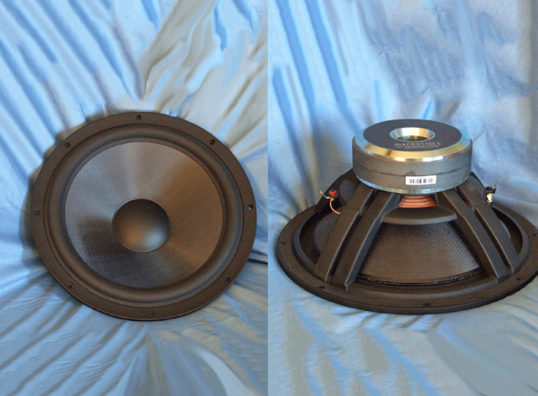
All this is driven by a 75.6 mm diameter (3”) four layer voice coil wound with round copper wire on a nonconducting fiberglass former. The motor system powering the cone assembly utilizes two stacked 20-mm thick by 180-mm diameter ferrite magnets sandwiched between a polished 8-mm thick front plate and a polished shaped 10-mm tall T-yoke that incorporates a 50-mm diameter pole vent. Two sets of braided voice coil lead wires terminate to a pair of gold-plated terminals.
I began characterizing the new SB42FHCL75-6 15” subwoofers with the LinearX LMS analyzer and VIBox. I generated the voltage and the admittance (current) measurements in free air at 1, 3, 6, 10, 15, 20, and 30 V. It should also be noted that this multi-voltage parameter test procedure includes heating the voice coil between sweeps for progressively longer periods to simulate operating temperatures at that voltage level (raising the temperature to the third time constant).
I further processed the 14 sine wave sweeps for each woofer sample with the voltage curves divided by the current curves to produce impedance curves. I used a highly accurate LEAP phase calculation routine to generate the phase curves. Then, I copy/pasted the impedance magnitude and phase curves plus the associated voltage curves into the LEAP 5 software’s Guide Curve library.
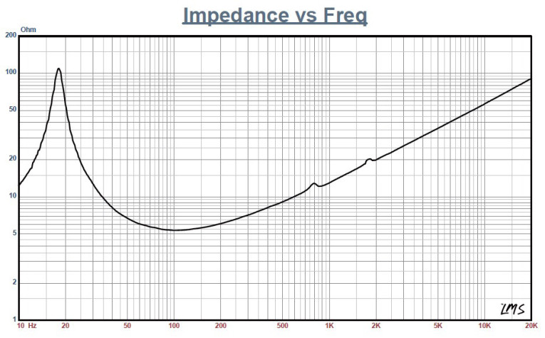
I used this data to calculate parameters using the LEAP 5 LTD transducer model. Because most manufacturing data is produced using either a standard transducer model, or in many cases the previous LEAP 4 TSL model, I also generated LEAP 4 TSL model parameters using the 1 V free air that can also be compared with the manufacturer’s data. Figure 1 shows the SB42FHCL75-6’s 1 V free-air impedance plot. Table 1 compares the LEAP 5 LTD and LEAP 4 TSL Theile-Small (T-S) parameter sets for the SB42FHCL75-6 driver samples along with the SB Acoustics factory data.
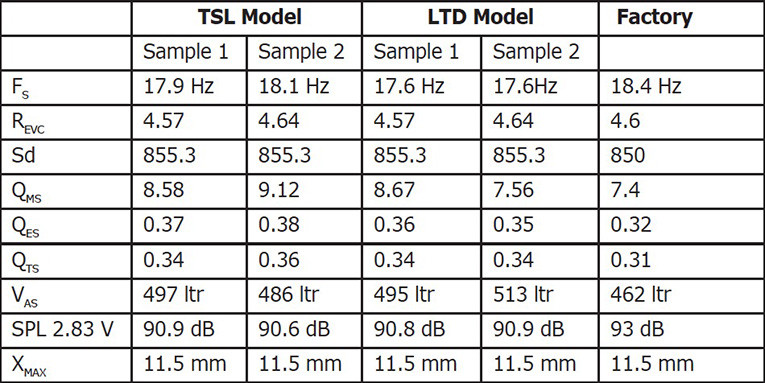


The comparative data shown in Table 1 shows all four parameter sets for the two samples were reasonably similar, with a small deviation in the sensitivity numbers. However, programming the factory data into LEAP and performing a sealed-box simulation resulted in the exact same F3 as the LTD Sample 1 data. I then took the Sample 1 LEAP 5 LTD parameters and set up two computer box simulations—one in a 4.75-ft3 Butterworth-type sealed enclosure with 50% fill material (fiberglass) and the other in a Quasi Third–Order Butterworth (QB3) vented box alignment in a 7.68-ft3 box with 15% fill material and tuned to 20 Hz.
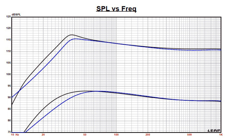
Figure 2 gives the results for the SB42FHCL75-6 in the sealed and vented enclosures at 2.83 V, and at a voltage level sufficiently high enough to increase cone excursion to 13.2 MM (XMAX + 15%).
This resulted in a F3 of 36 Hz (–6 dB = 28.2 Hz) with a QTC = 0.7 for the 4.75-ft3 closed box and a –3 dB for the QB3 vented simulation of 27 Hz (–6 dB = 22 Hz). Increasing the voltage input to the simulations until reaching the approximate XMAX +15% maximum linear cone excursion point resulted in 115.5 dB at 43.5 V for the sealed enclosure simulation and 117.2 dB with a 48-V input level for the larger vented box. Figure 3 shows the 2.83 V group delay curves. Figure 4 shows the 43.5 V/48 V excursion curves.
Klippel analysis for the SB42FHCL75-6 produced the Klippel data shown in Figures 5–8. (Our analyzer is provided courtesy of Klippel GmbH and the testing was performed by Patrick Turnmire, Redrock Acoustics. For more information, visit www.redrockacoustics.com).
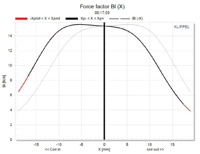
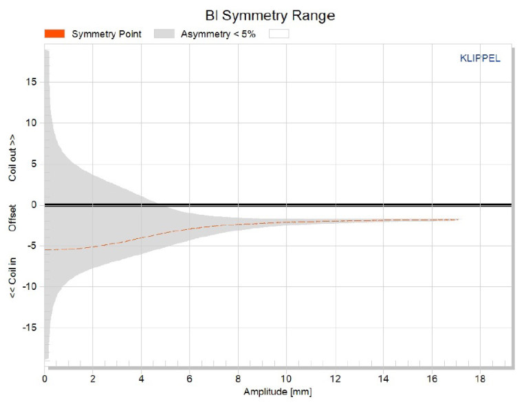
The SB42FHCL75-6’s Bl(X) curve shown in Figure 5 is broad and moderately symmetrical with a slight tilt typical of a driver with substantial XMAX. The Bl symmetry curve depicted in Figure 6 shows 5.4 mm Bl coil-in (rearward) offset at rest (also an area of higher uncertainty), which transitions to a 2 mm coil-in offset at about 8.3 mm of excursion, where it remains constant through out the rest of the excursion range.
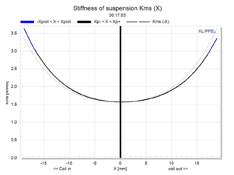
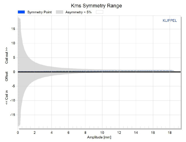
Figure 7 shows the KMS stiffness of compliance curve, which is very symmetrical and does not exhibit any offset at all. Figure 8 shows the KMS symmetry range curve, which indicates practically no offset, with only a very slight coil-out offset at the driver’s physical XMAX of about 0.4 mm. The SB42FHCL75-6’s displacement limiting numbers calculated by the Klippel analyzer using the subwoofer criteria for Bl was XBl at 70% (Bl dropping to 70% of its maximum value) equal to greater than 109 mm (somewhat lower than the driver’s physical 11.5 mm XMAX) for the prescribed 20% distortion level (the criterion for subwoofers).
For the compliance, crossover (XC) at 50% CMS minimum was greater than 16.7 mm (substantially greater than the driver’s physical XMAX), which means the Bl is the more limiting factor for getting to the 20% distortion level. For a subwoofer where 20% distortion is not really perceivable, this is good performance.
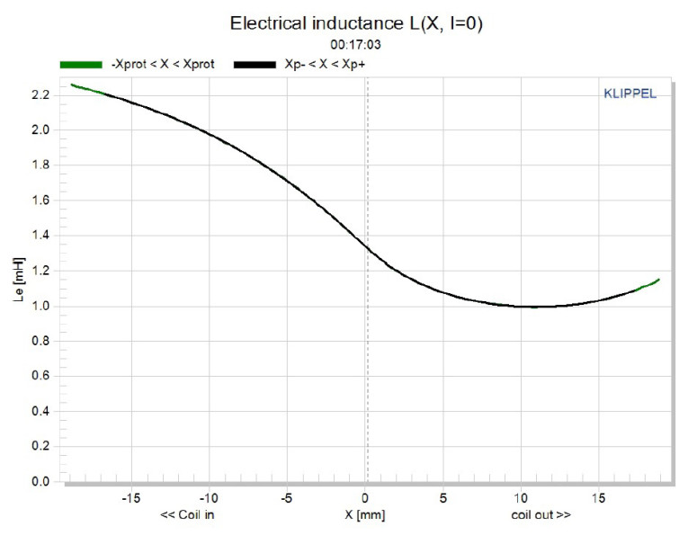
Figure 9 gives the inductance curve Le(X) for this transducer. Motor inductance will typically increase in the rear direction from the zero rest position and decrease in the forward direction as the voice coil moves out of the gap and has less pole coverage, which is exactly what happens here. The range of inductance swing is about 1 mH from XMAXIN to XMAXOUT. My only comment might be that you could probably achieve better detail and definition by limiting this amount of inductance with an appropriate shorting ring, which I’m sure SB Acoustics could easily accommodate on request.
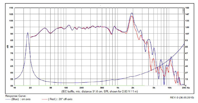
Normally, I mount the driver in a box and measure the on- and off-axis SPL. However, I generally do not do this for subwoofers, as they usually crossover over at 100 Hz or lower. Regardless, Figure 10 gives the factory SPL and as can be seen, it would certainly be possible to cross this device as high as any 15”, likely somewhere between 300–800 Hz.
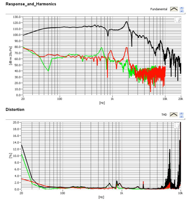
Next, I used the Listen SoundCheck analyzer to perform distortion analysis. I dispensed with time-frequency analysis for subwoofers, as the data is not really significant below 100 Hz. For distortion measurements, I set the voltage level with the driver mounted in a free air and increased the voltage until the driver produced a 1 m SPL of 94 dB (4.34 V), which is my SPL standard for home audio driver distortion measurement. The distortion measurement was then made with the microphone placed near-field (10 cm) from the center point of the cone (see Figure 11). This actually includes two plots, the top graph being the standard fundamental SPL curve with the second and third harmonic curves, and the bottom graph the second and third harmonic curves, plus the total harmonic distortion (THD) curve with an appropriate X-axis scale.
Interpreting the subjective value of conventional distortion curves is almost impossible. However, looking at the relationship of the second to third harmonic distortion curves is of value. As can be inferred from the data, this is a well-designed subwoofer transducer from SB Acoustics (which includes design work from Danesian Audio). For more information, visit www.sbacoustics.com. VC
This article was originally published in Voice Coil, April 2016.