Recently, there has been increased demand for loudspeaker 3-D directivity measurements both in the near- and far-fields. For example, in home audio, the Consumer Electronics Association’s “Standard Method of Measurement for In-Home Loudspeakers” (CEA-2034) specifies a “spinorama” test in which the results are presented in ways to help interpret how a loudspeaker might sound in an average listening room.
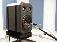
Professional PA equipment requires accurate complex directivity data in the far-field. Studio reference monitors and today’s personal audio devices are designed to be used in the near-field. Traditional measurement techniques have significant drawbacks in accuracy, cost, and space. So, the question is how to overcome these drawbacks to satisfy the new requirements. New holographic near-field scanning techniques provide new ways to determine the sound pressure at any point in the 3-D sound field. This article explores and compares traditional measurements against this new technique using the Dayton Audio ES140Ti-8 woofer as the device under test (DUT) sample mounted in a sealed box.
Traditional Loudspeakers
Measurement loudspeakers are measured in the far-field where the sound pressure decays by 6 dB per double the distance. To avoid ambient noise and reflected sound, the measurement should be performed under free-field conditions. However, due to climate conditions, this is not always practical. Therefore, anechoic chambers were developed where the influences of reverberant sound, ambient noise, climate, and varying air temperature distributions are negligible. Another possible method is to simulate free-field conditions. This involves gating (windowing) of the impulse response, which suppresses room reflections at higher frequencies.
Far-field measurements using traditional methods have significant drawbacks in accuracy, cost, and space. Measurement accuracy depends on room dimensions (low frequencies), far-field microphone placement, and air temperature deviations (phase errors). No anechoic room is perfect. They suffer from limited absorption at low frequencies and they also exhibit absorption irregularities. In addition, anechoic chambers are expensive and require permanent installation. For simulated free-field measurements, the low-frequency resolution is limited by the time difference between the direct sound and the first reflected sound.
For traditional 3-D directivity measurements in the far-field, angular resolution is determined by the number of measurement points, which may become impractical at high resolutions. Reducing the number of measurement points using weighted spatial averaging introduces estimation errors.
Benefits of Near-Field Measurements
In the near-field, the velocity and sound pressure are out of phase and as a consequence the inverse square law does not apply. Therefore, the sound pressure cannot be extrapolated into the far-field. However, this is no longer a negating factor, which I will explain later in this article. The high signal-to-noise ratio (SNR) in the near-field allows the measurement to tolerate some ambient noise from the environment. The direct sound’s amplitude is much larger than the reflected sound’s amplitude leading to good free-field simulated conditions. The near-field also reduces the possibility of phase errors from variations in air temperature.
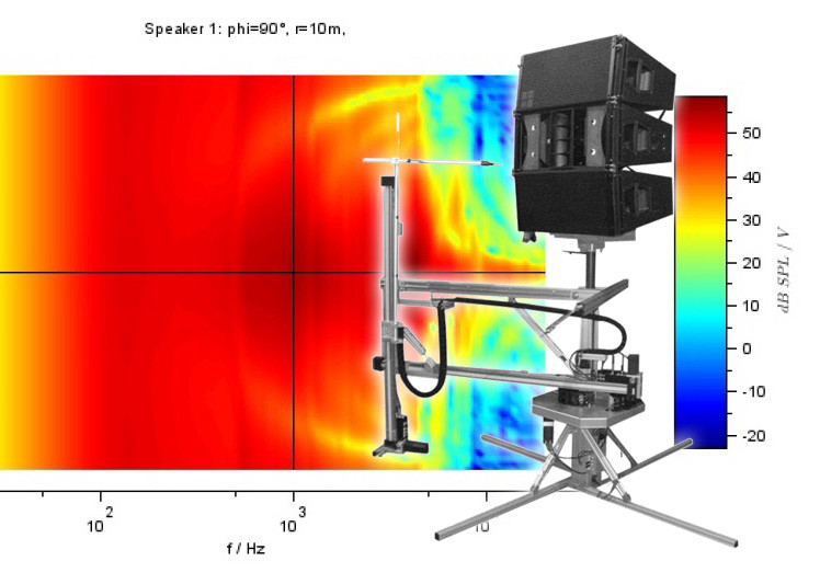
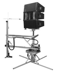
Recently, Klippel of Dresden, Germany, introduced its Near-Field Scanner (NFS), which is revolutionizing loudspeaker measurements (see Photo 1). The NFS makes a holographic measurement of the sound pressure in the near-field to generate a set of coefficients that accurately determine the sound pressure at any point in the 3-D sound field outside the scanning surface.
By exploiting the advantages of near-field measurements and using spherical harmonic wave expansion, the near-field sound pressure can be extrapolated into the far-field. The near-field scanning process can produce a true free-field measurement because the outgoing wave (direct sound) can be separated from the incoming wave (reflected sound).
Room dimensions and acoustical treatments are not a factor for eliminating the need for large expensive anechoic chambers. Directivity and other far-field characteristics can also be derived from the near-field information. The wave expansion process facilitates high spatial resolution using fewer measurement points. Measurements derived from post processing are faster and more comprehensive than traditional directivity measurement methods.
Scanning Process in the Near-Field
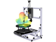
Using robotics, the microphone rotates around the loudspeaker measuring the sound pressure distribution on a cylindrical surface. In this way, the loudspeaker has constant interaction with the room and the microphone position can be accurately determined. In addition, stationary loudspeakers are easier to support with minimal gear—a big advantage for anyone measuring large heavy loudspeakers. To facilitate field separation, two thinly separated cylindrical surfaces are scanned. A double-layer scan provides information about the incoming and outgoing sound waves that can be used to separate the direct sound from the room reflections, providing free field conditions.
Spherical Harmonic Wave Expansion
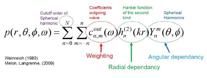
An expansion into spherical waves can be represented by a series of basic Hankel and spherical harmonic functions in which each function is weighted by a complex coefficient. The complete set of coefficients describes the loudspeaker’s characteristics (see Figure 1). These coefficients are used to reconstruct the transfer function, which is used to determine the sound pressure at any point outside the scanning surface both in the near- and far-fields.
As the sound field’s frequency and complexity increases, the order of the expansion also needs to increase. The coefficients are complex and frequency dependent. The number of coefficients required is (N+1)2 where N is the highest order in the expansion. Truncating the order has the effect of smoothing the
directional properties (lobes).
measurement applications.
Measurement Point Requirements
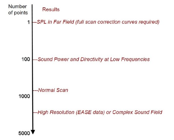
The required number of measurement points depends on the required number of coefficients, which in turn depends on the order of the expansion that accurately represents the 3-D sound field. The required order of expansion depends on the sound field’s complexity, the resolution of the application, and the measurement environment (i.e. field separation requirements).
The sound field’s complexity depends on the size of loudspeaker, the number of transducers, and the axial symmetry. Figure 2 shows the number of measurement points required to yield a specific result. At low frequencies, the sound field has limited complexity and can be characterized with just a few basic functions. So, a small number of measurement points are required.
Measurement Accuracy and the Maximum Order of Expansion
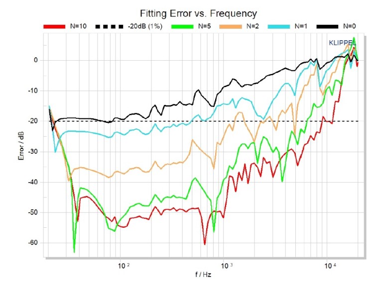
Figure 3 shows the fitting error vs. frequency for different orders of the wave expansion N = 0, 1, 2, 5, and 10. The fitting error indicates potential problems such as poor SNR, insufficient order, or geometrical errors in the scanning. The number of measurement points is always more than the number of required coefficients. This redundancy is the basis for calculating the fitting error. An order of N = 10 provides a good fitting error up to 10 kHz (shown by the red curve in Figure 3).
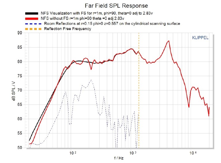
Figure 4 is a sound pressure level (SPL) comparison using the NFS under non-anechoic conditions where the black curve shows the Dayton ES140Ti-8 processed using field separation and the red curve shows it processed without field separation. The dashed blue curve is the room reflections measured at the reference point on the cylinder scanning surface. Notice how the peaks and the dips in the reflection curve line up with the peaks and the dips in the red curve.
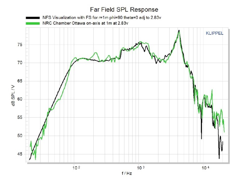
Near-field scanning that includes field separation can remove the room modes in a reverberant environment and an anechoic environment! It is truly a free-field measurement. In Figure 5, the peaks at 100, 210, and 320 Hz clearly show the insufficient damping in the anechoic chamber. The non-anechoic room’s dimensions are approximately 4.2m × 3.9m × 4.2m. The National Research Council (NRC) chamber was pre-manufactured with a claimed low cut-off frequency of 85 Hz and dimensions of 15.2m × 8.8m × 6.7m. To purchase this chamber today would cost approximately $500,000. The NFS setup used for this test costs roughly one-fifth of that.
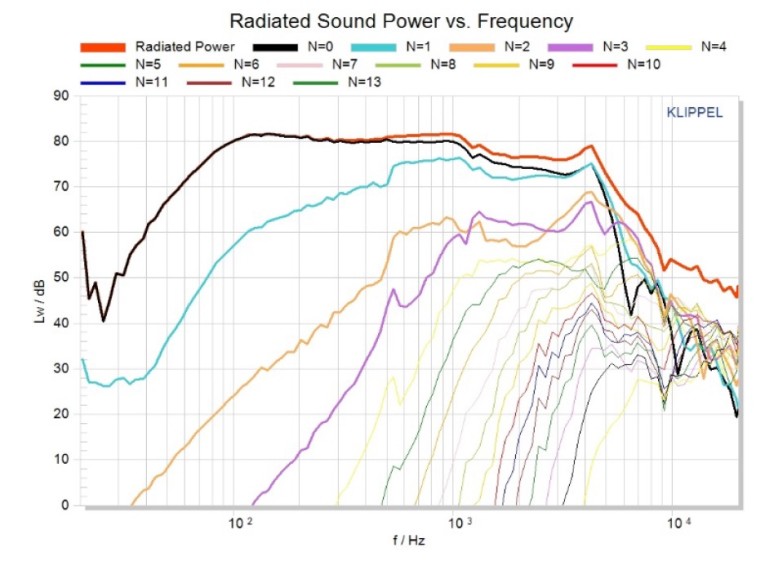
Figure 6 shows the radiated sound power curve vs. frequency. The sound power associated with each order N contributes to the total sound power. As the frequency increases, the order of the expansion needs to increase and the amount of sound power contributed by each order becomes more significant. In this example, N = 0 almost completely describes the sound power between 20 and 200 Hz. This indicates that only a minimal amount of measurement points (100 points in an anechoic environment) are required to produce the total sound power curve at low frequencies. On average, the NFS will take approximately 20 min to perform this measurement.
Few Measurement Points Required
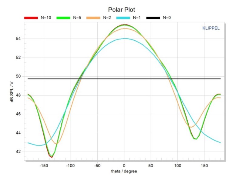
Significant data reduction occurs when the measurement points are converted into coefficients. Wave expansion interpolates between the measurement points. Therefore, the required number of measurements points is much lower than the angular resolution of the calculated directivity pattern. Figure 7 shows the 2-D polar plots in the far-field (10 m) at 1 kHz for orders N = 0, 1, 2, 5, and 10 with a 5° resolution. Notice that the sound field at 1 kHz is completely described by order 5 (i.e., the green curve closely matches the red curve).
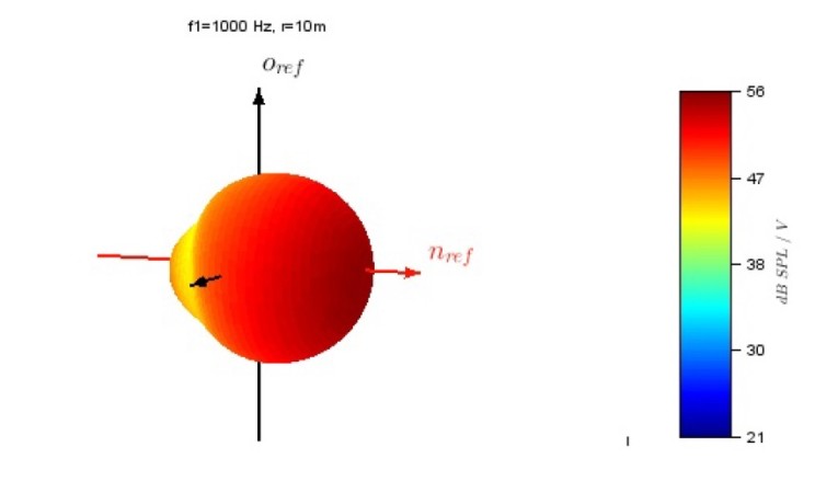
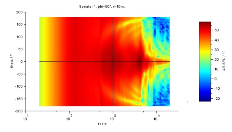
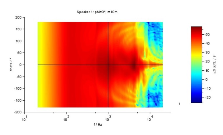
This measurement was performed under non-anechoic conditions using field separation. The directivity can also be viewed in 3-D using balloon plots. Figure 8 shows a balloon plot at 1 kHz in the far-field (10 m), while Figure 9 shows the directivity vs. frequency in the horizontal plane. Figure 10 shows the directivity vs. frequency in the vertical plane. These contour plots are used to determine the SPL’s uniformity in their respective planes.
Other Possible Measurements
The results from the NFS can be used to satisfy the requirements of the “spinorama” test from CEA-2034. For PA applications requiring accurate phase information at high frequencies, the data from a high-resolution scan can be exported to EASE. The NFS can also be used to make single-point measurements in the nearfield that can be extrapolated into the far-field. This is useful for quick SPL checks when modifying crossovers or transducers, provided the type and the position of the loudspeaker does not change. The process requires correction curves generated from a full scan compared against a single-point measurement in the near-field.
In Summary
Holographic Measurement of the 3-D sound field using Near-Field Scanning provides the following benefits:
• More information about the acoustical output (near-field and far-field)
• Sound pressure at any point outside the scanning surface in the near- and far-fields (complete 3-D space)
• Improved accuracy compared to conventional far-field measurements (coping with room reflections, microphone positioning, gear reflections, air temperature variations, etc.)
• Higher angular resolution with less measurement points
• Simplified handling (rotating the microphone instead of heavy loudspeakers)
• Dispenses with an anechoic room and far-field measurements
• Self-check capability by evaluating the fitting error
• Comprehensive data set with low redundancy
• Not a permanent installation
• Considerably less expensive than an anechoic chamber. For more information on the new Klippel NFS and the services provided by Warkwyn Associates, visit www.klippel.de and www.warkwyn.com
This article was originally published in Voice Coil, May 2015.