To determine the input impedance of a device, you must know both the voltage across the device and the current flowing into the device. The impedance is simply the voltage across the device, E, divided by the current flowing into it, I. This is given by the following equation:
Z = E/I [1]
You should understand that because the voltage, E, and the current, I, are complex quantities, the impedance, Z, is also complex. That is to say impedance has a magnitude and an angle associated with it.
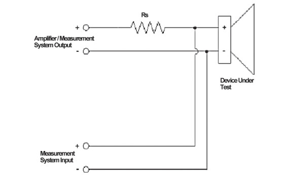
When measuring loudspeaker input impedance, it is common today for many measurements to be made at relatively low drive levels. This is necessary because of the method employed in the schematic of Fig. 1. In this setup a relatively high value resistor, say 1kΩ, is used for Rs. As seen from the input of the DUT, it is being driven by a high impedance constant-current source. Had it been connected directly to the amplifier/measurement system output, it would in all likelihood be driven by a low impedance constant voltage source. In both of these cases constant refers to there being no change in the driving quantity (either voltage or current) as a function of frequency or load.
When Rs is much larger than the impedance of the DUT, the current in the circuit is determined only by Rs. If the voltage at the output of the amplifier, Vo, is known, this current is easily calculated with the following equation and is constant.
Is = Vo/Rs [2]
Now that you know the current flowing in the circuit, all you need to do is measure the voltage across the DUT and you can calculate its input impedance.
There is nothing wrong with this method. It is limited, as previously mentioned, however, in that the drive level exciting the DUT will not be very large due to the large value of Rs. For some applications this may be problematic.
Loudspeakers are seldom used at the low drive levels to which we are limited using this method. It may be advantageous to be able to measure the input impedance at drive levels closer to those used in actual operation.
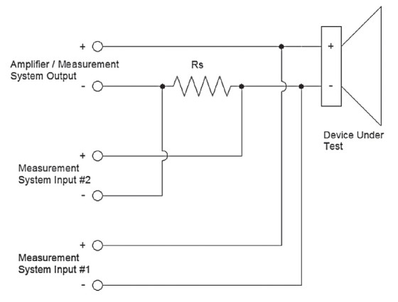
If you can measure the current in the circuit rather than having to assume it is constant, you can avoid this limitation. Using a measurement system with at least two inputs, as shown in Fig. 2, can do just that. In this case Rs is made relatively small, say 1Ω or less. This is called a current sensing resistor, or also a current shunt. Technically, this is incorrect for this application, because a current shunt is always in parallel with a component from which current is diverted. The voltage drop across Rs is measured by input #2 of the measurement system. The current in the circuit is then calculated using the equation
Is = Vs/Rs [3]
The voltage across the DUT is measured by input #1 of the measurement system. You now know both the voltage across and the current flowing into the DUT, so you can calculate its input.
I used EASERA for the measurements in this article. It has facilities for performing all of these calculations, as should most dual channel FFT measurement systems. As Fig. 2 shows, you should set channel #1 across the DUT as the measurement channel, and channel #2 as the reference channel. Dual channel FFT systems divide the measurement channel by the reference channel, so you have
Result = Channel #1/Channel #2
= VDUT/Vs
By substitution from Equation 3:
Result = VDUT/(Is*Rs)
Because Z = VDUT/Is it follows that
Z = Result * Rs or Z = Rs * Channel #1/Channel #2
All you need to do is multiply the dual channel FFT measurement by the value of Rs used and you get the correct value for impedance. If you choose Rs to be 1.0Ω, this becomes really easy.
In EASERA there is not an Ohm display selection. Selecting a Volt display will yield the correct values for the displayed curve. For other measurement systems this may work as well, but it is recommended to check the display by measuring a known resistor value for proper calibration.
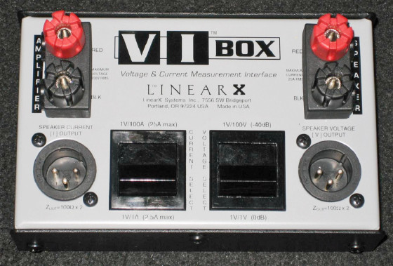
A very useful device for performing impedance measurements using this current sensing resistor method is the VI Box from LinearX (www.linearx.com). The signal from the amplifier is routed through the VI Box, which contains the current sensing resistor, and then onto the DUT (Fig. 3). It actually contains two selectable sensing resistors, 1Ω and 10mΩ (milli-Ohm), which allow for measurements using a greater range of current supplied to the load (DUT). The voltage across the selected resistor is present across pins 2 and 3 of one of the XL connectors. The voltage across the DUT is present across pins 2 and 3 of the other XL connector. These connectors allow for quick and easy interface with balanced inputs of a computer/audio interface (sound card). There is also a selectable voltage divider so the input of the audio interface won’t be overloaded when testing with very high voltage.
I mentioned previously that measuring input impedance at low drive levels may present a problem for some applications. A couple of these that come to mind are vented loudspeaker enclosures and constant voltage distributed system transformers. I’m sure the interested reader will find others.
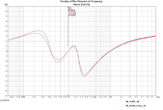

The impedance response of a vented loudspeaker enclosure is shown in Fig. 4. The angle of the impedance for this device is shown in Fig. 5. The vent tuning resonance of this loudspeaker is found when the impedance angle is zero indicating the voltage and current are in phase. This is denoted by the marker at approximately 98Hz. These graphs show measurements using both the constant-current method with a 1kΩ resistor and using a current sensing resistor. The current sensing resistor measurement used a 0dBV (1.0V) drive level to excite the loudspeaker. There is some difference between these two measurements.
The impedance measurements in Fig. 6 tell us much more. In this graph you have additional measurements at +18, +24, and +27dBV. You can see that at these higher drive levels the impedance curve changes rather dramatically.
The vent surface area of this loudspeaker is relatively small compared to the surface area of the driver. When the woofer is driven harder, it moves much more air. The vents are too small to allow this same volume of air to be moved through them.
The vents saturate. As more air attempts to move through the vents, they saturate more and have less of an effect on the loudspeaker response. The impedance response begins to look less like a vented box and more like that of a sealed box.
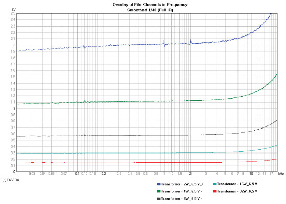
A constant voltage distributed loudspeaker system typically requires transformers to be placed immediately in front of the loudspeakers to step down the voltage and step up the current. Testing these types of transformers at low voltage levels typically will not reveal some of the problems that may occur in actual usage. Figure 7 shows the input impedance for each primary tap of a 70.7V step-down transformer with its secondary loaded by an 8Ω power dissipation test resistor. For each of these measurements the drive voltage was 6.5V. This is approximately -21dB from the full rated voltage of 70.7V.
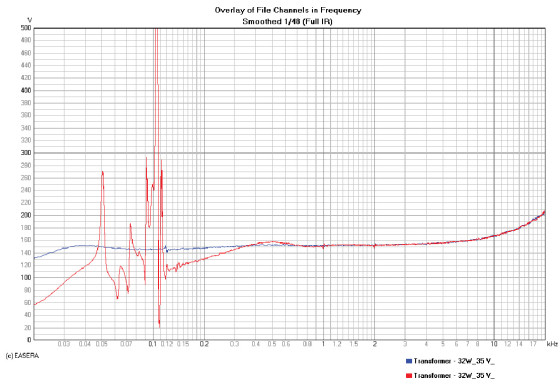
As expected, the impedance curves are fairly well behaved. When driven at 35V, -6dB from full rated voltage, there is a problem with the 32W tap seen in Fig. 8. At very low frequencies this transformer does not like being driven at this voltage. The result is that the core saturates. The reflected impedance of the load (on the secondary) as seen by the primary is no longer linear. This violates one of the requirements of the measurement method used (FFT); that the DUT be linear, time invariant (LTI).
By placing a second-order Butterworth high-pass filter in front of the amplifier driving the transformer, you can correct this core saturation condition. A doubling of voltage to 70V would require the corner frequency of the high-pass filter to also be doubled. In this case, the corner frequency should be increased from 30Hz to 60Hz.
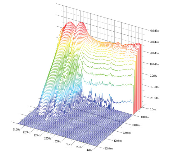
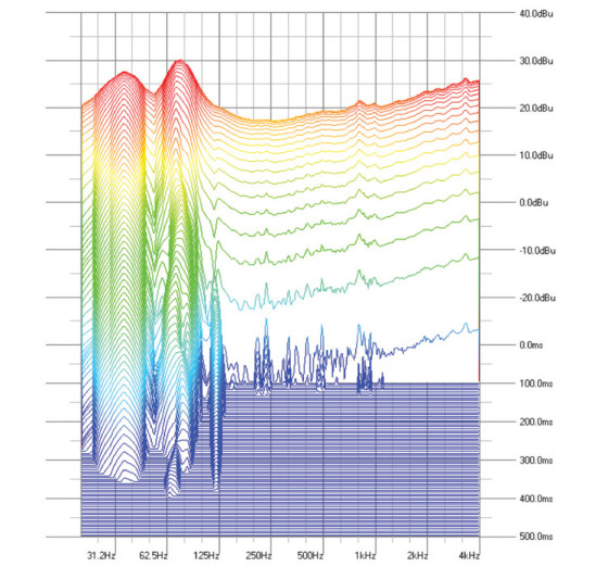
Another use for these types of measurements is to investigate resonance behavior. This can be particularly interesting when viewed as a 3D waterfall. The impedance response of a vented enclosure is shown in Fig. 9. Note the dip/peak at 80 and 120Hz, as well as these same frequency regions in Figs. 10 and 11. These features don’t occur initially. It is only after approximately 60ms that they become evident. Knowing how long it requires for this resonance to develop may help in determining its cause and implementing a solution.
I hope that this method that measures impedance at typical application drive level and shows some possible uses will be of benefit. Thanks to Jay Mitchell (Frazier Loudspeakers) and Dr. Eugene Patronis (Professor Emeritus, Physics—Georgia Institute of Technology) for their insights on some of these applications.
Ed. Note — Voice Coil began using the LinearX VI Box to do constant-current source multiple voltage impedance measurements in the October 2003 Test Bench column. This was required to utilize the advanced modeling technique offered by the LinearX LEAP 5 LTD transducer model. Coincidentally, that was the same month that we began using Klippel data in Test Bench!
This article was originally published in Voice Coil, February 2011.