In this test-bench I analyzed the Tymphany Peerless 3.5” diameter SLS-85S25CP-04-04 (see Photo 1). This mini-woofer is extensively used in TV soundbars, pedestal soundbars (soundbars that contain down firing subwoofers that double as a TV stand), docking stations/Bluetooth powered speakers, and desktop speakers (e.g., the Sonos products, Jambox, Beats, Samsung, Bose and many others). For two-way applications in these categories, this SLS-85S25CP-04-04 is a good example of what works.
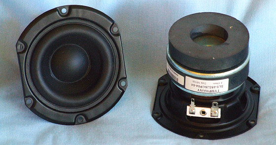
The SLS-85S25CP-04-04 is built on a proprietary stamped frame that is fully vented below the spider mounting shelf for enhanced cooling. The cone assembly consists of a black paper cone with a black paper 35-mm diameter dust cap. Both are suspended with a black styrene-butadiene rubber (SBR) surround and a cloth flat spider (damper). For a 3.5” driver, the SLS-85S25CP-04-04 has a fairly standard 1” diameter voice coil wound with round copper wire on a KSV non-conducting former, which is terminated to a set of solderable terminals.
Driving the cone assembly is a 15-mm × 72-mm ferrite magnet with a bump-out T-yoke that has a secondary bucking magnet on top of the bump-out. This is used to increase Bl, as there is a maximum available diameter limited by the mounting hole size for the driver. There is also an aluminum shorting ring (Faraday Shield) on the pole piece for distortion reduction.
I used the LinearX LMS analyzer and VIBox to create voltage and admittance (current) curves with the SLS-85S25CP-04-04 clamped to a rigid test fixture in free air at 0.3, 1, 3, 6 and 10 V. I discarded the 10-V curves as being too nonlinear for LEAP 5 to get a good curve fit. I no longer use a single added mass measurement. Instead, I use actual measured mass, which is the manufacturer’s measured Mmd data.
Next, I post-processed the four 550-point stepped sine wave sweeps for each of the SLS-85S25CP-04-04 samples. I divided the voltage curves by the current curves (admittance) to produce the impedance curves, phase generated by the LMS calculation method. I imported the information, along with the accompanying voltage curves, to the LEAP 5 Enclosure Shop software.
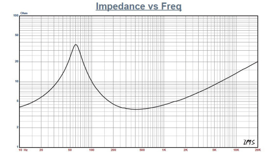
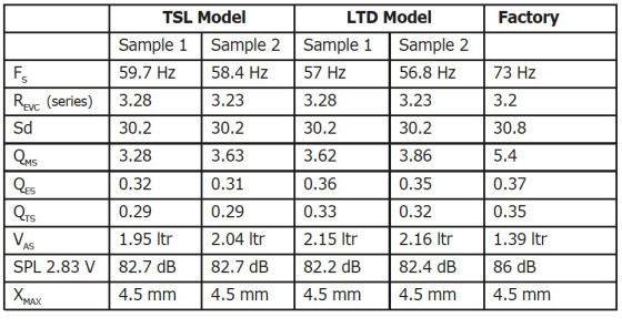
Since most T-S data provided by OEM manufacturers is produced using a standard method or the LEAP 4 TSL model, I used the 1-V free-air curves to additionally create a LEAP 4 TSL model. I selected the complete data set, the LTD model’s multiple voltage impedance curves, and the TSL model’s 1-V impedance curve in the transducer derivation menu in LEAP 5 and created the parameters for the computer box simulations. Figure 1 shows the 1-V free-air impedance curve. Table 1 compares the LEAP 5 LTD and TSL data and factory parameters for both SLS-85S25CP-04-04 samples.
There is definitely some variation between my measurements and the factory parameters. The factory numbers were high for the VAS and the sensitivity. However, the factory data’s enclosure simulations were not far off the curves from my data, except for sensitivity.
Next, I followed my usual protocol and used the LEAP LTD parameters for Sample 1 to set up computer enclosure simulations. I programmed two computer enclosure simulations into LEAP—a 40-in3 QB3 vented box alignment (with 15% damping material in the box) tuned to 70.8 Hz and a 74-in3 EBS-type vented alignment tuned to 57 Hz (with 15% damping material).
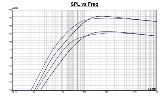
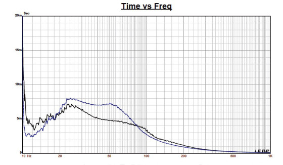

Figure 2 displays the SLS-85S25CP-04-04’s results in the two box simulations at 2.83 V and at a voltage level high enough to increase cone excursion to 5.2 mm (XMAX + 15%). This produced a F3 frequency of 103 Hz (F6 = 83.5 Hz) for the 40-in3 QB3 vented enclosure and –3 dB = 85.6 Hz (F6 = 64.4 Hz) for the 74-in3 EBSvented simulation.
I increased the voltage input to the simulations until the maximum linear cone excursion was reached, which resulted in 96 dB at 9 V for the F3 enclosure simulation and 95 dB with the same 9-V input level for the EBSvented enclosure. Figure 3 and Figure 4 show the 2.83-V group delay curves and the 9-V excursion curves, respectively.

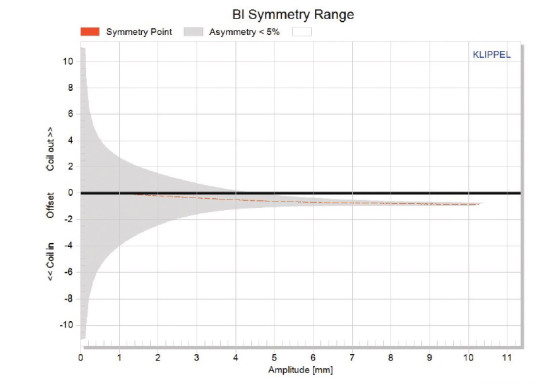
Figures 5–8 show the SLS-85S25CP-04-04’s Klippel analysis and testing results. Patrick Turnmire performed the testing, which produced the Bl(X), KMS (X) and Bl and KMS symmetry range plots. Figure 5 shows the SLS-85S25CP-04-04’s Bl(X) curve, which is moderately broad and fairly symmetrical. Figure 6 shows the SLS-85S25CP-04-04’s Bl symmetry plot and the offset at rest is nearly zero, progressing to a small coil-in offset of only 0.57 mm at the driver’s physical XMAX.
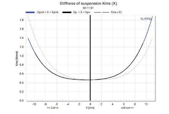
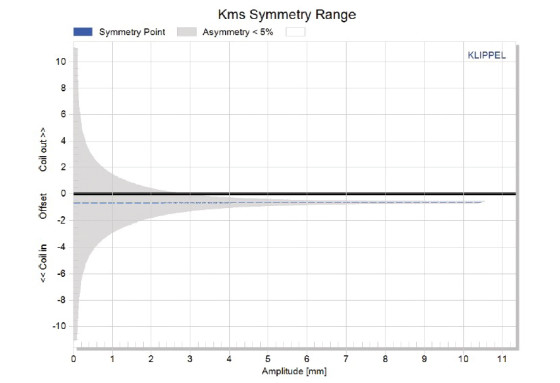
The SLS-85S25CP-04-04’s KMS (X) and KMS symmetry range curves are shown in Figure 7 and Figure 8. The KMS (X) curve is also rather symmetrical and has a minor rearward (coil-in) offset of about 0.65 mm at the rest position. It remains constant out to the physical XMAX position. The SLS-85S25CP-04-04’s displacement limiting numbers were XBl at 82%. The Bl is 5.8 mm for the XC at 75%. The CMS minimum was 5.4 mm, which means that for the SLS-85S25CP-04-04, both compliance and Bl are greater than the physical XMAX prescribed 10% distortion level.
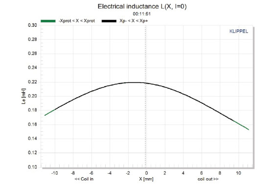
Figure 9 shows the SLS-85S25CP-04-04’s inductance curve Le(X). Inductance will typically increase in the rear direction from the zero rest position as the voice coil covers more pole area, which is not what happens with the SLS-85S25CP-04-04’s inductance. Instead, the inductance decreases in both directions (coil-in and coil-out) with a small variation of only 0.02 mH maximum from the XMAXIN AND XMAXOUT positions, which is good and mostly due to the aluminum shorting ring.
Next, I mounted the SLS-85S25CP-04-04 in an enclosure that had a 5” × 10” baffle filled with damping material (foam). Then, I used the LinearX LMS analyzer set to a 100-point gated sine wave sweep. I measured the transducer on- and off-axis from 300 Hz to 20 kHz with the frequency response at 2.83 V/1 m.
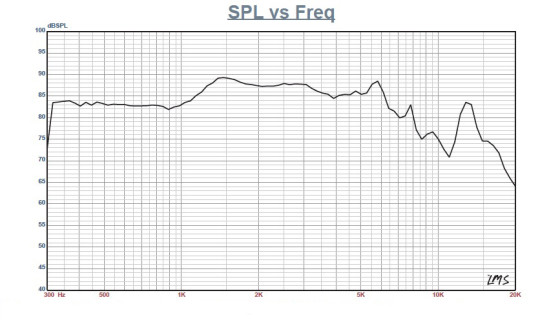
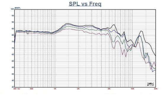

Figure 10 shows the SLS-85S25CP-04-04’s on-axis response, indicating a relatively anomaly-free response to about 6 kHz, with a 6-dB shelf between 1 and 1.5 kHz. Figure 11 shows the on- and off-axis frequency response at 0°, 15°, 30°, and 45°. Looking at the on-axis compared to the 30° off-axis curve, and using –3 dB as a criterion, a crossover frequency anywhere between 3 to 5 kHz should produce a good power response for a two-way system design. Figure 12 shows the SLS-85S25CP-04-04’s two sample SPL comparison, which is a close match to 3 kHz and within 1 to 2 dB for 3 kHz and above.
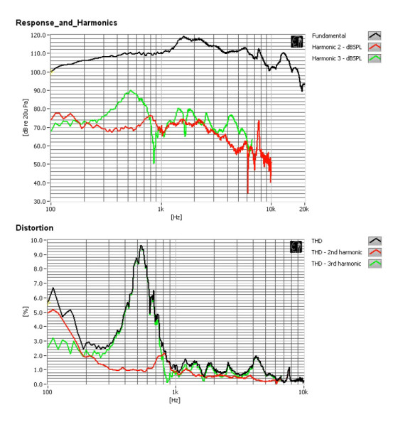
For the remaining tests, I used a Listen SoundCheck AmpConnect analyzer with a Listen 0.25” SCM microphone and a power supply to measure distortion and generate time-frequency plots. For the distortion measurement, I mounted the SLS-85S25CP-04-04 in free-air and used a noise stimulus to set the SPL to 94 dB at 1 m (7.4 V) I measured the distortion with the microphone placed 10 cm from the dust cap. Figure 13 shows the distortion curves.
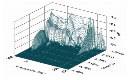
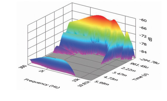
I used SoundCheck for a 2.83-V/1-m impulse response for the SLS-85S25CP-04-04 and imported the data into Listen’s SoundMap time-frequency software. Figure 14 shows the resulting CSD waterfall plot. Figure 15 shows the Wigner-Ville plot. The SLS-85S25CP-04-04 — when used in its intended applications (e.g., in small two-way designs, or TV, multimedia, and lifestyle speakers) — should work quite well.
www.tymphany.com
This article was originally published in Voice Coil August 2104.