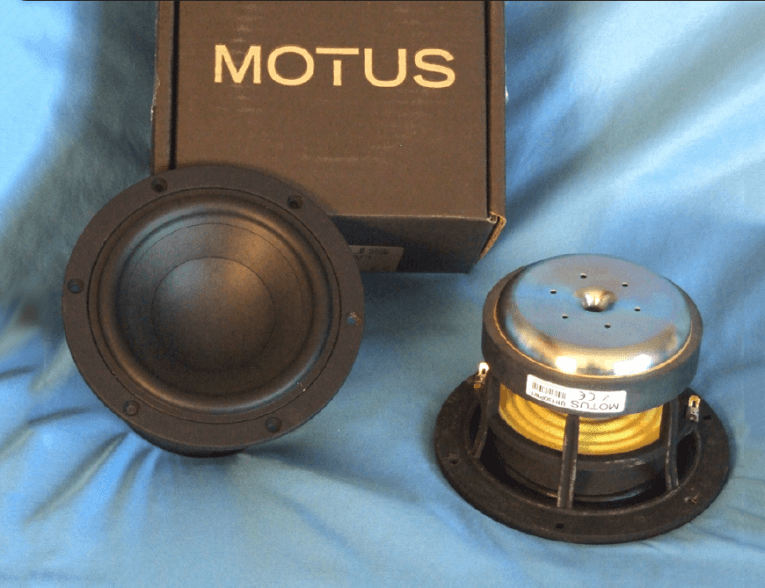
Motus Audio drivers are designed by US transducer engineers and built in China, which is starting to be more common among high-end audio manufacturers, with companies such as Revel, Monitor Audio, and Sonus Faber sourcing out of China and Indonesia. Voice Coil did its first review of a Motus Audio product, the Motus Audio UH25CTI dome tweeter, in the December 2012 issue, followed by the Motus Audio UH205P1 8” mid-bass driver featured in the November 2015 issue. This month, Motus Audio sent me the 5.25” version of its woofer line, the UH130PW1 (see Photo 1).
The feature set for the UH130PW1, has a similar feature set as several other European high-end mid-bass woofer brands. Starting with the frame, Motus used a nicely configured six-spoke cast-aluminum frame with narrow 11 mm wide spokes to minimize reflections back into the cone. The area below the suspended spider mounting shelf is almost completely open, resulting in effective cooling of the motor and the voice coil. For the cone assembly, Motus chose a rather stiff curvilinear profile pressed paper cone with a fairly large (reinforcing almost at the midpoint of the cone) 2.5” diameter concave pressed paper dust cap. Compliance is provided by an nitrile-butadiene rubber (NBR) surround, designed with a shallow discontinuity where it attaches to the cone edge to minimize cone-edge breakup. Remaining compliance comes from a 3.75” diameter flat cloth spider.
The FEA optimized motor design for the UH130PW1 is well thought-out and incorporates a ferrite ring magnet, a machined undercut pole piece, and dual copper shorting rings (Faraday shields). Like the Scan-Speak Illuminator series woofers, the UH130PW1 has an underhung gap design with an 8 mm winding height in an 18 mm gap.
This drives a 1.75” (44.2 mm) diameter four-layer voice coil wound with round copper wire on a non-conducting Kapton former. Motor parts above and below the 110 mm × 20 mm magnet are machined and polished. Additional cooling is provided by an 8 mm diameter rear pole vent plus six 3 mm diameter peripheral vents. Last, the voice coil is terminated to a pair of gold-plated terminals appropriately located on opposite sides of the frame. In terms of the overall physical appearance, the UH130PW1 is an impressive looking mid-bass transducer!
I began analysis of the UH130PW1 using the LinearX LMS analyzer and VIBox to create voltage and admittance (current) curves. The driver was clamped to a rigid test fixture in free air at 0.3, 1, 3, 6, 10, 15, and 20 V. As with most 5.25” diameter woofers, 15 V curves are usually too nonlinear for LEAP to get a reasonable curve fit and usually have to be discarded. However, due to the UH130PW1’s linearity and high XMAX, I was able to get a usable curve fit on the 15 V curves.
I did have to discard the 20 V curves, but that’s still impressive for a 5.25” diameter driver. As per the established measurement protocol for Test Bench, I turned the LMS oscillator on for a progressively increasing time period between sweeps to keep the driver heated as close to the third thermal time constant as possible (from 10 to 50 seconds between sweeps, depending on the voltage level).
Under Test Bench testing protocol, I no longer use a single added mass measurement to determine VAS. Instead, I use the actual measured cone assembly mass (Mmd) supplied by the driver manufacturer, which was 14.85 grams for the Motus Audio 5.25” woofer. Next, I post-processed the 12 550-point stepped sine wave sweeps for each UH130PW1 sample and divided the voltage curves by the current curves (admittance) to derive impedance curves, phase added by the LMS calculation method.
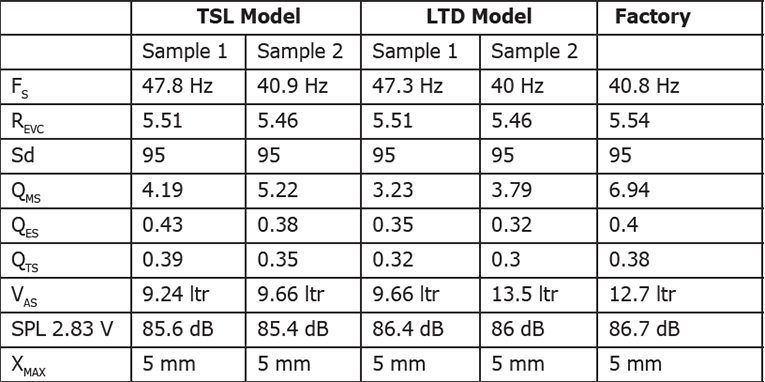
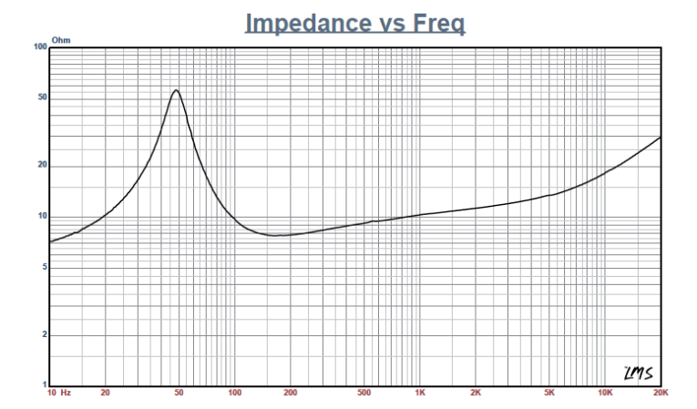
I imported them, and along with the accompanying voltage curves, to the LEAP 5 Enclosure Shop software. Since most Thiele-Small (T-S) data provided by the majority of OEM manufacturers is generated using either the standard model or the LEAP 4 TSL model, I additionally created a LEAP 4 TSL parameter set using the 1 V free-air curves. I selected the complete data set, the multiple voltage impedance curves for the LTD model, and the 1 V impedance curve for the TSL model in the LEAP 5 transducer derivation menu and created the parameters for the computer box simulations. Figure 1 shows the 1 V free-air impedance curve. Table 1 compares the LEAP 5 LTD, TSL, and factory published parameters for both of Motus UH130PW1 samples.
The UH130PW1’s LEAP parameter calculation results were reasonably close to the published factory data, although the TSL was closer. As usual, I set up computer enclosure simulations using the LEAP LTD parameters for Sample 1. I programmed two computer box simulations into LEAP 5—one was a Butterworth sealed enclosure with a 210 in3 volume with 50% fiberglass damping material and a QB3 vented enclosure with a 346 in3 volume tuned to 49 Hz with 15% fiberglass fill material.
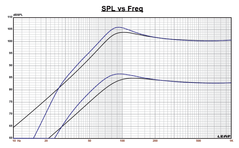
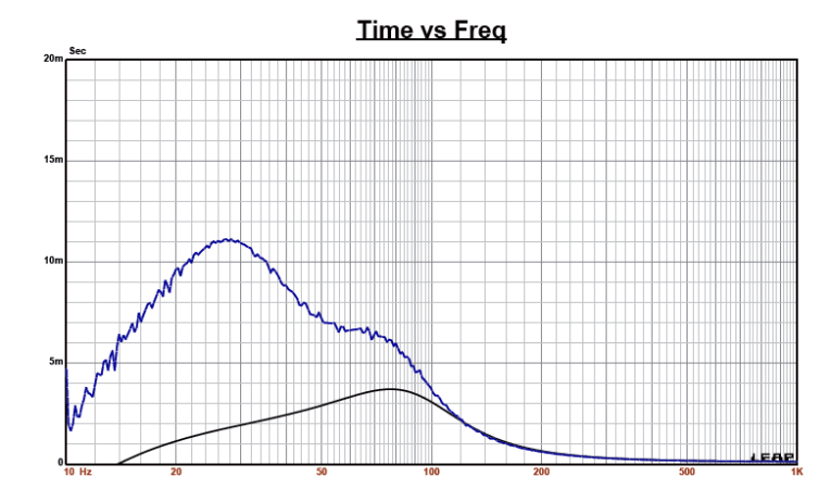
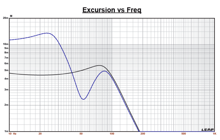
Figure 2 displays the UH130PW1’s results in the sealed and vented boxes at 2.83 V and at a voltage level sufficiently high enough to increase cone excursion to 5.75 mm (XMAX + 15%). This produced a –3 dB = 76 Hz (F6 = 62 Hz) with a QTC = 0.68 for the sealed box, and for the QB3 vented enclosure a F3 frequency of 65 Hz (F6 = 54 Hz). Increasing the voltage input to the simulations until the maximum linear cone excursion was reached resulted in 104 dB at 30 V for the sealed enclosure simulation and 106 dB for the same 30 V input level for the larger vented box. Figure 3 shows the 2.83 group delay curves. Figure 4 shows the 30 V excursion curves.
Because the vented box example reached maximum excursion at about 40 Hz, a steep 24 dB/octave high-pass active filter located about 30 to 35 Hz would increase the power handling and output the vented box example. The UH130PW1’s Klippel analysis produced the Bl(X), KMS(X), and Bl and KMS symmetry range plots shown in Figures 5–8. (Our analyzer is provided courtesy of Klippel GmbH and Patrick Turnmire of Redrock Acoustics performs the analysis. This data is extremely valuable for transducer engineering, so if you would like to have analysis done, visit www.redrockacoustics.com.)
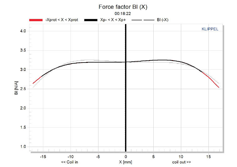
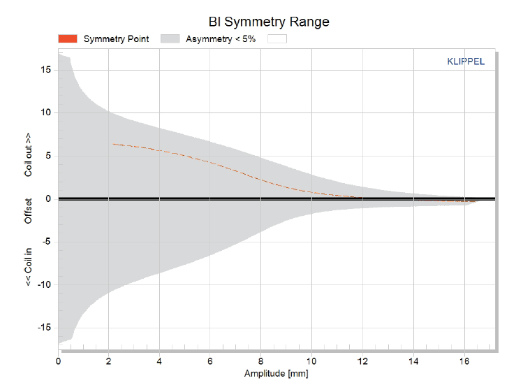
The UH130PW1’s Bl(X) curve is reasonably symmetrical and shows quite a broad Bl curve for a 5.25” woofer, which is typical of an underhung motor (see Figure 5). Looking at the Bl symmetry plot, the curve in Figure 6 shows a substantial amount coil-out offset at 4 mm of excursion, but that is in a region of high uncertainty for the analyzer. Even though the UH130PW1’s physical XMAX is 5 mm. The region of much higher certainty extends out to beyond 10 mm, which is also an affectation of underhung motors on the Klippel analyzer.
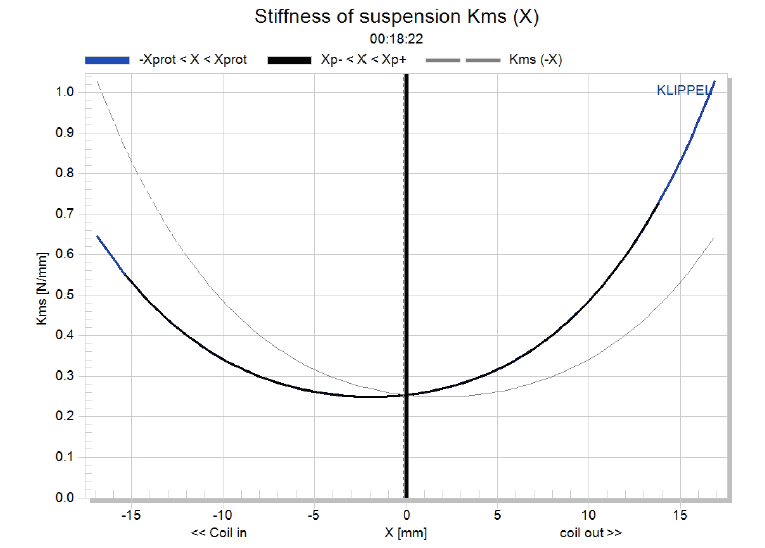
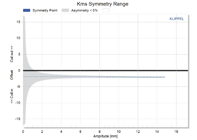
Figure 7 shows the UH130PW1’s KMS(X) curve is not as symmetrical in both directions as the Bl curve. Figure 8 shows the UH130PW1’s KMS symmetry range curves, which has fairly small coil-out offset at the rest position (1.9 mm). This is fairly constant throughout the operating range, possibly suggesting the coil position in the gap needs some minor adjustment on this sample. The UH130PW1’s displacement limiting numbers calculated by the Klippel analyzer were XBl at 70% Bl = 5.8 mm and for crossover (XC) at 75% CMS minimum was 3.9 mm, which means the compliance is the most limiting factor for distortion level of 20%.
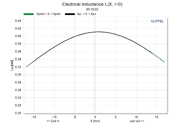
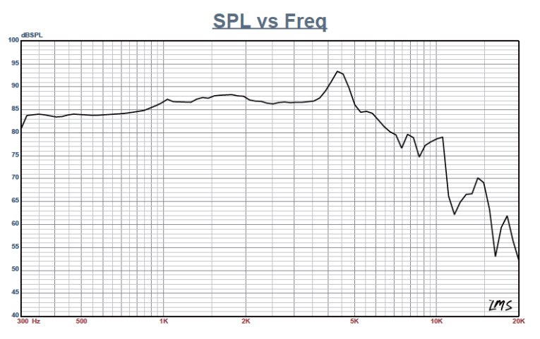
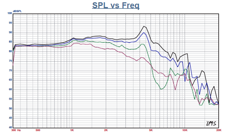
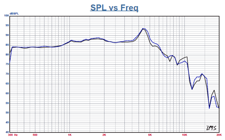
Figure 9 gives the UH130PW1’s inductance curves Le(X). Inductance will typically increase in the rear direction from the zero rest position as the voice coil covers more pole area. However, inductance does not occur because of the effective multiple copper inductive shorting rings (Faraday shields). What you see as a result is a fairly minor inductance swing with inductive variation of only 0.05 mH from the resting position to the in and out XMAX positions, which is very good inductive performance.
With the Klippel testing completed, I mounted the UH130PW1 in an enclosure that had a 15” × 7” baffle and was filled with damping material (foam). Then, I used the LinearX LMS analyzer set to a 100-point gated sine wave sweep to measure the device under test (DUT) on and off axis from 300 Hz to 20 kHz frequency response at 2.83 V/1 m. Figure 10 shows the UH130PW1’s on-axis response, indicating a smoothly rising response to about 4 kHz, where it begins is low-pass roll-off. Figure 11 displays the on- and off-axis frequency response at 0°, 15°, 30°, and 45°. The –3 dB frequency at 30° off axis relative to the on-axis sound pressure level (SPL) is about 1.9 kHz, suggesting a crossover between 2 kHz should be appropriate. And finally, Figure 12 gives the UH130PW1’s two-sample SPL comparisons, showing a close match throughout the operating range up to 4 kHz.
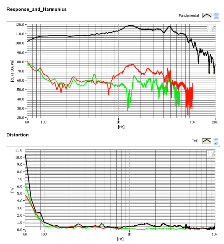
For the remaining series of tests, I employed the Listen SoundCheck software, AmpConnext analyzer, and SCM microphone (all courtesy of Listen, Inc.) to measure distortion and generate time-frequency plots. For the distortion measurement, I rigidly mounted the UH130PW1 in free air, and placed the SPL set to 94 dB at 1 m (6.7 V) using a noise stimulus. Then, I measured the distortion with the Listen microphone placed 10 cm from the dust cap. Figure 13 shows the distortion curves.
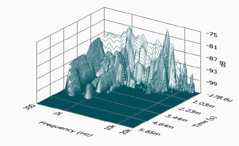
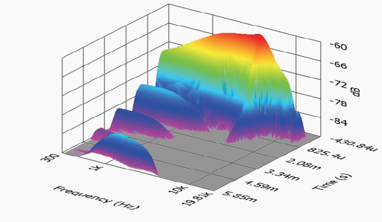
I then used SoundCheck to get a 2.83 V/1 m impulse response and imported the data into Listen’s SoundMap Time/Frequency software. Figure 14 shows the resulting CSD waterfall plot. Figure 15 shows the Wigner-Ville (for its better low-frequency performance) plot. For more information, visit www.motusaudio.com
This article was originally published in Voice Coil, January 2016.