

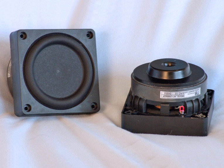


The W3-2088SOF is built on an injection-molded eight-spoke frame that supports an unusual rectangular housing. The really unusual feature is that the W3-2088SOF does not use a spider. Instead it gets its compliance from two surrounds. Photo 1 shows the surround glued to a flat diaphragm. Underneath this rectangular structure is another surround and flat diaphragm spaced about 0.25” apart from each other, but with the surround roll in the reverse direction, like a dual spider configuration to cancel out odd-order nonlinearities. The voice coil former is vented below the inside diaphragm and also vented between the two diaphragm.
The W3-2088SOF is driven by a 32-mm diameter (1.25”) voice coil wound with round copper wire on a paper-reinforced vented aluminum former. The motor system that powers the cone assembly utilizes a single 15-mm thick 82-mm diameter ferrite magnet sandwiched between a 4-mm thick black-coated front plate and a black-coated shaped T-yoke that incorporates a 15-mm diameter pole vent. Last, the braided voice coil lead wires end at a pair of solderable terminals mounted on opposite sides of the frame.
I used the LinearX LMS analyzer and VIBox to begin characterizing the new W3-2088SOF. I generated the voltage and admittance (current) measurements in free-air at 0.3, 1, 3, 6, and 10 V. Surprisingly, at least for a 3.5” diameter driver, the device remained linear enough to obtain a good curve fit at 10 V. (Most drivers this small do not stay linear enough to use voltage higher than 6 V.)
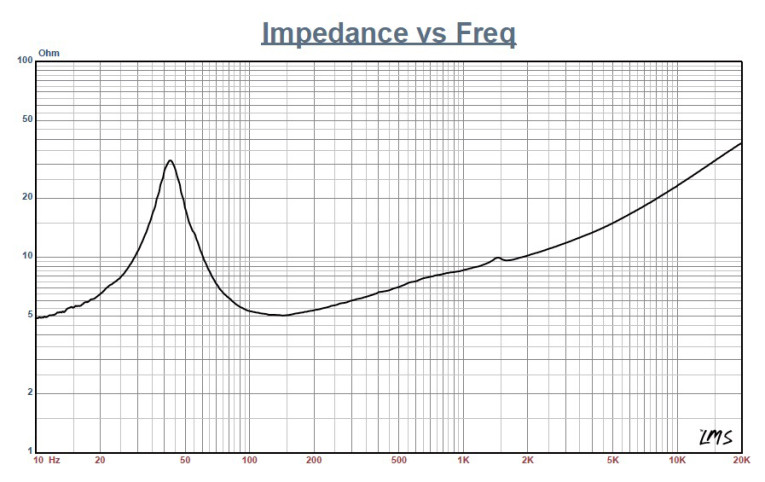
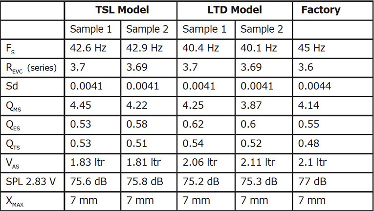
I divided the voltage curves by the current curves to produce impedance curves and further processed each woofer sample’s 10 sine wave sweeps. I used the LEAP phase calculation routine to generate phase curves for each impedance curve. Then, I copy/pasted the impedance magnitude and phase curves plus the associated voltage curves into the LEAP 5 software’s Guide Curve library. I used this data to calculate parameters with the LEAP 5 LTD transducer model. Because almost all manufacturing Thiele-Small (T-S) parameter data is produced using either a standard transducer model or in many cases the LEAP 4 TSL model, I also used the 1-V free-air curves to generate LEAP 4 TSL model parameters. Figure 1 shows the W3-2088SOF’s 1-V free-air impedance plot. Table 1 compares the W3-2088SOF’s LEAP 5 LTD and LEAP 4 TSL T-S parameter sets driver samples along with the Tang Band factory data.
From the W3-2088SOF’s comparative data, it is apparent that all four parameter sets for the two samples were reasonably similar and correlated well with the factory data.
Following my normal Test Bench testing protocol, I used the sample 1 LEAP 5 LTD parameters and set up two computer box simulations. I used a 126.6-inch3 Butterworth-type sealed enclosure with 50% fill material (fiberglass) for the first simulation. For the second simulation, I used a vented box Chebychev/Butterworth alignment in a 209.4-inch3 box with 15% fill material and tuned to 31.4 Hz.
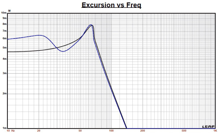
Figure 2 shows the W3-2088SOF’s results in the sealed and vented enclosures at 2.83 V and at a voltage level high enough to increase cone excursion to 8.1 mm (XMAX + 15%). This resulted in a F3 of 57 Hz (–6 dB = 46.5 Hz) with a Qtc = 073 for the 126.6 inch3 closed box and a –3 dB for the Chebychev/Butterworth vented simulation of 46 Hz (–6 dB = 35 Hz). Increasing the voltage input to the simulations until the approximate XMAX + 15% maximum linear cone excursion point was reached resulted in 94.5 dB at 15 V for the sealed enclosure simulation and 96 dB with a 15.25 V input level for the larger vented box. Figure 3 and Figure 4 show the 2.83-V group delay curves and the 15-V/15.25-V excursion curves.
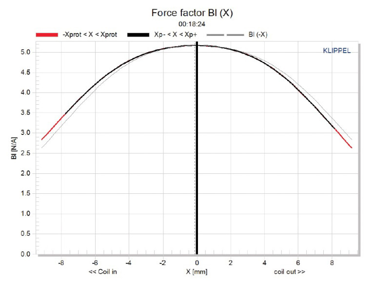
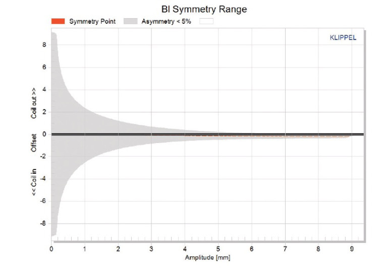


The W3-2088SOF’s Klippel analysis produced the Klippel data graphs shown in Figures 5–8. Figure 5 shows the W3-2088SOF’s Bl(X) curve is a very broad and symmetrical curve typical of a driver with substantial XMAX (7 mm is a large XMAX for a 3.5” driver). The Bl symmetry curve shown in Figure 6 reveals virtually no offset for this driver. Figure 7 and Figure 8 show the W3-2088SOF’s KMS(X) and KMS symmetry curves.
Figure 7 shows that, as with the Bl curve, the W3-2088SOF’s KMS stiffness of compliance curve is very symmetrical, with only a minor coil-out offset. The KMS symmetry range curve has a minor 0.34-mm coil-out offset at rest remaining constant to the W3-2088SOF’s physical XMAX.
The W3-2088SOF’s displacement limiting numbers calculated by the Klippel analyzer using the subwoofer criteria for Bl was XBl at 70% (Bl dropping to 70% of its maximum value) equal to 7 mm for the prescribed 20% distortion level. For the compliance, crossover at 50% CMS minimum was 6 mm (1 mm less than the W3-2088SOF’s physical XMAX), which means compliance is the more limiting factor to get the 20% distortion level.

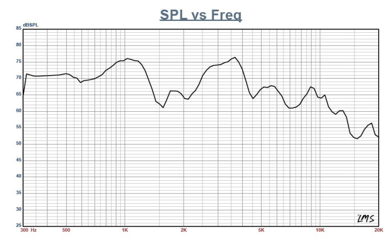
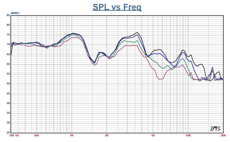
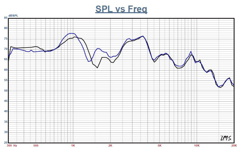
Figure 9 shows the W3-2088SOF’s inductance curve Le(X). Motor inductance typically increase in the rear direction from the zero rest position and decrease in the forward direction as the voice coil moves out of the gap and has less pole coverage. The W3-2088SOF’s inductance curve Le(X) shows a typical response. However, the inductive change is a minimal 0.1 mH from the rest position to XMAX in either direction.
After the Klippel analysis, I mounted the W3-2088SOF in an enclosure filled with foam damping material that had a 12” × 5” baffle area. I used the LMS gated sine wave technique to measure the W3-2088SOF’s SPL on- and off-axis. Figure 10 shows the on-axis response measured 300 Hz to 20 kHz at 2.83 V/1 m. Even though the response was pretty ragged, you should be able to cross this driver up to 800 Hz if required. Figure 11 shows the on- and off-axis to 45° and confirms this. Finally, Figure 12 shows the two-sample SPL comparison. Given this is a subwoofer with a flat diaphragm, it is not really a problem.
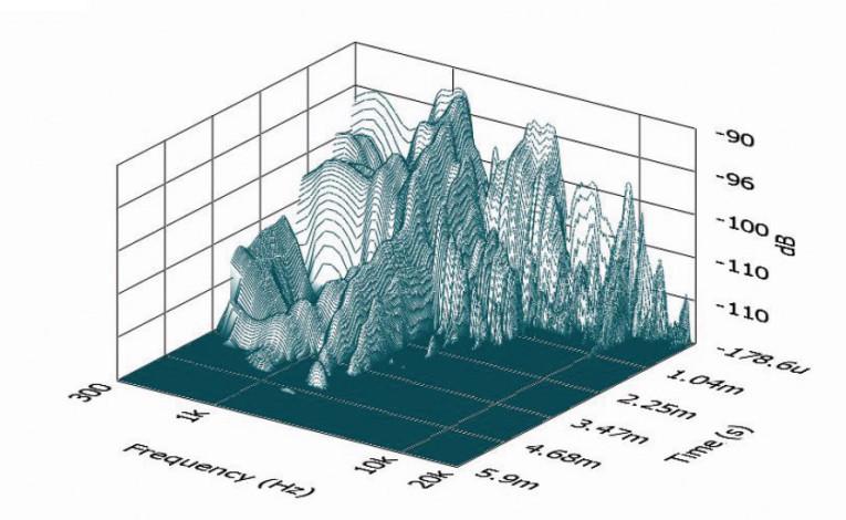
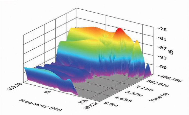
Next, I used the Listen SoundCheck analyzer to perform distortion analysis. I normally dispense with time-frequency analysis for subwoofers as the data is not really significant below 100 Hz. However, since W3-2088SOF could be crossed higher than that, I included the measurements. With the woofer still mounted in a foam damped enclosure with a 8” × 12” baffle, I used SoundCheck to make an impulse measurement. I imported the data into Listen’s SoundMap software, windowed to remove the room reflections, and produced the waterfall plot shown in Figure 13. The Wigner-Ville plot is shown in Figure 14.
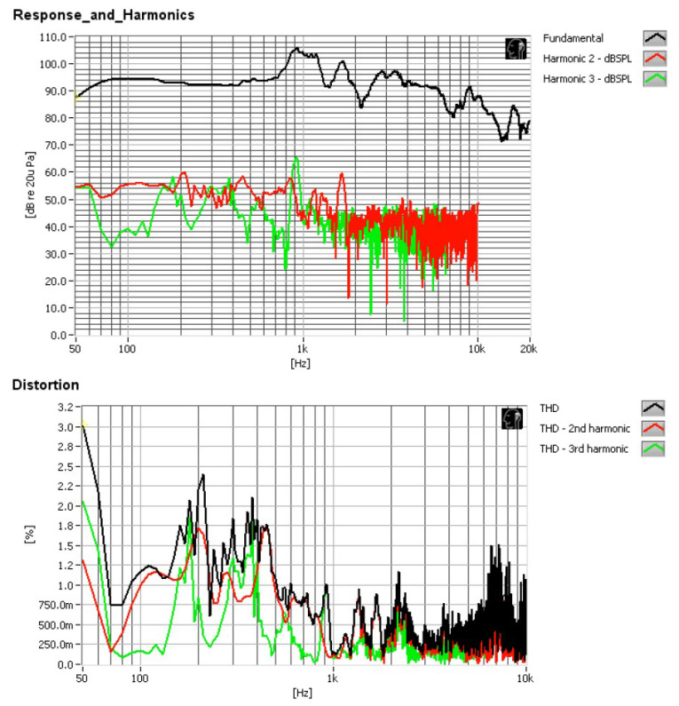
For the distortion measurements I set the voltage level with the driver mounted in free air and rigidly attached to a fixture. I used pink noise to increase the voltage until it produced a 1-m SPL of 94 dB (10 V), which is my SPL standard for home audio drivers. I measured the distortion with the microphone placed nearfield (10 cm) with the woofer mounted in the enclosure (see Figure 15). The results are actually shown in two plots. Figure 15a shows the standard fundamental SPL curve with the second- and third-harmonic curves. Figure 15b shows the second- and third-harmonic curves plus the THD curve with an appropriate X-axis scale.
Interpreting the subjective value of conventional distortion curves is almost impossible; however, it is important to examine the second-harmonic distortion curve’s relationship to the third-harmonic distortion curve.
The W3-2088SOF is a uniquely conceived (when was the last time you saw a spider-less woofer with dual surrounds and diaphragms?) and good-performing mini subwoofer from Tang Band. For more information, visit www.tb-speaker.com. VC
This article was originally published in Voice Coil, January 2014.
