Directional queues come from the first arrival response. We judge arrival direction in well under a millisecond. However, judging what we are hearing takes longer. To determine spectral balance, the ear/brain combination analyzes the incoming sound typically over a 5 to 30ms interval. This interval is called the Haas fusion zone. Within this interval we are not aware of reflected sounds as separate spatial events. All of the sound appears to come from the direction of the first arrival. Lateral reflections from adjacent walls help extend the soundstage beyond the physical span of the loudspeakers. The comb filtering action of the many early reflections arriving at the listening position with varying phases adds a sense of spaciousness to the sound. (It also argues against the need for phase accuracy in loudspeakers.)
You can see that the perceived timbres of sounds in rooms are the result of temporal processing and spatial averaging of reflected sounds arriving at our ears from many angles. In typical home listening rooms, direct sound and early reflected sounds dominate. Late reflections are greatly attenuated. This is clear from the measurement of RT60s in the range of 0.2 to 0.4 seconds. (Compare this to concert halls where RT60s of 3 to 4 seconds are common.) What we hear is a function of the directional characteristics of the loudspeakers and strong early reflections from the room boundaries.
You can think of the early reflection response as a loudspeaker’s in-room response averaged over a period extending out to 30ms after first arrival. But now we have a problem. The early reflection response is room dependent. A designer cannot predict how the early reflection response will look in any particular room. This will depend on the room size and shape and speaker location. It will also be affected by the room furnishings, any acoustic treatment, and the number of people in the room.
However, we can examine a loudspeaker’s directional characteristics anechoically. To guarantee that sound arriving at the listening position is affected only by the arriving reflections and not by any off-axis anomalies in the speaker’s response, the off-axis response curves should be smooth replicas of the on-axis response with the possible exception of some rolloff at higher frequencies and larger off-axis angles.
Polar Response
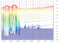
I have found that the best way to represent a loudspeaker’s off-axis response is with a 3D waterfall plot, which is assembled by measuring a speaker’s off-axis response at a number of equally spaced angles. The polar data is used to determine the listening window, early reflection, and power responses. DAAS generates a 3D polar waterfall response automatically in conjunction with a computer-controlled turntable.
In the polar waterfall option DAAS performs a sequence of measurements. Between each measurement DAAS sends a control signal to the turntable to move a specified number of degrees. The full range of measurement is 180°. Figure 14 is a polar waterfall plot for my example loudspeaker. To obtain this plot the speaker was rotated in the horizontal plane from 90° left of on-axis to 90° right of the on-axis position in 10° increments. Except for a gentle rolloff at higher frequencies and larger angles, the off-axis curves are excellent replicas of the on-axis curve. You can see that the off-axis response curves are smooth replicas of the on-axis response with the expected rolloff at higher frequencies and larger off-axis angles due to the narrowing polar response of the tweeter. The high-frequency rolloff produces the desired listening window and early reflection responses of Fig. 1 in part 1.
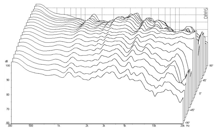
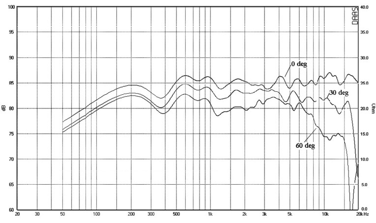
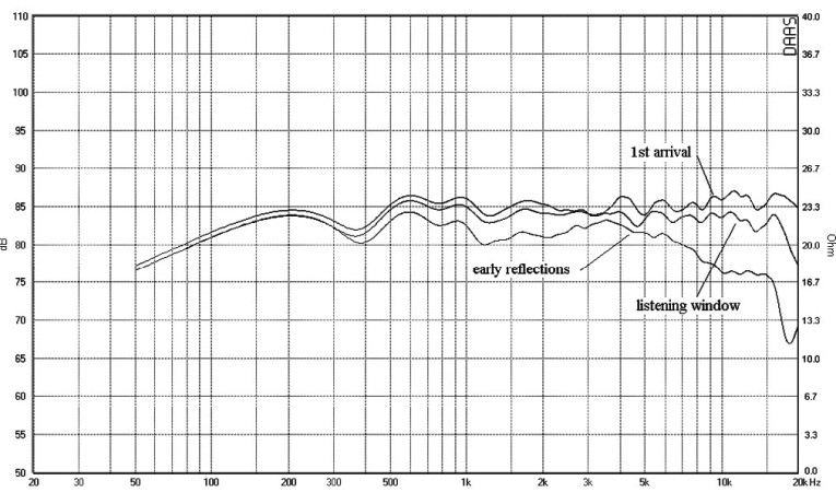
Figure 14 gives an excellent qualitative view of polar response performance, but reading actual values off the plot is difficult. Using the polar data collected for Fig. 14, I have plotted on-axis response and off-axis responses at 30° and 60° in Fig. 15. You can see that the 28mm tweeter response falls fairly quickly above 8kHz at 60° off-axis.
Using the polar response data, you can estimate the listening window and early reflection responses. I determined the listening window response by averaging on-axis response with off-axis responses in 5° increments from 25° left to 25° right and between 10° up and 10° down. You can approximate the early reflection performance by averaging all responses in the horizontal plane. The results (shown in Fig. 16) agree rather well with the criteria of Fig. 1. The curves shown on this plot appear to have a great deal of ripple, but this is due to the choice of the plot scale. Actually, the on-axis response lies within a ±2dB window above 500Hz.
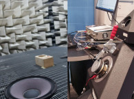
The power response is obtained by measuring responses at many locations over a spherical volume. This can only be done accurately in an anechoic chamber or, alternatively, in a totally reverberant enclosure. Because neither venue is available to me, I cannot show the power response for my example loudspeaker.
Step Response
Up to this point we have looked at loudspeaker performance solely in the frequency domain. Let’s turn now to the time domain for additional performance insight. We could examine the impulse response in more detail, but it is not easily interpreted. It is dominated by the tweeter response in the first few milliseconds. It doesn’t tell us much about the woofer, or the midrange if there is one, because all the low-frequency information is in the impulse response tail, which is at a very low signal level. The step response is a much more useful tool.
The step input is a signal that rises instantaneously from zero to a fixed level. This is basically a DC input starting at time zero. Mathematically, the step response is the time integral of the impulse response.
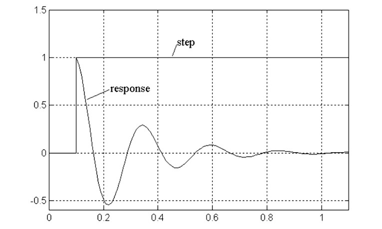
Figure 17 shows the response of an ideal loudspeaker to a step input. Loudspeakers are high-pass devices that cannot produce a static (i.e., DC) acoustic output. Therefore, the step response must drop below zero for a sufficient time to produce a net output of zero over time. The ideal step response is an exponentially decaying cosine wave oscillating at the fundamental resonant frequency of the loudspeaker.
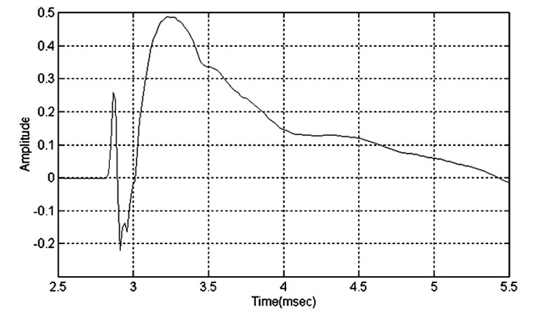
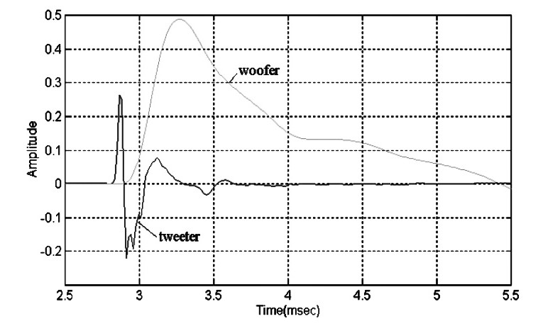
Figure 18 shows the step response for my example loudspeaker on an expanded time scale. The oscillatory portion of the response is not shown. This plot is actually a combination of two step responses: the initial sharp rise of the tweeter followed by the much slower broader rise of the woofer. This is shown more clearly in Fig. 19, where the tweeter and woofer step responses are plotted separately.
What can you tell from these plots? First, you see that both the tweeter and woofer are connected with positive polarity. Both initially rise in the positive direction. Next you see a smooth handoff from the tweeter to the woofer at roughly 3.1msec. This speaks well of the crossover design. Finally, from Fig. 18 you see that the speaker is not time coherent.
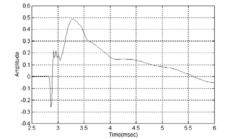
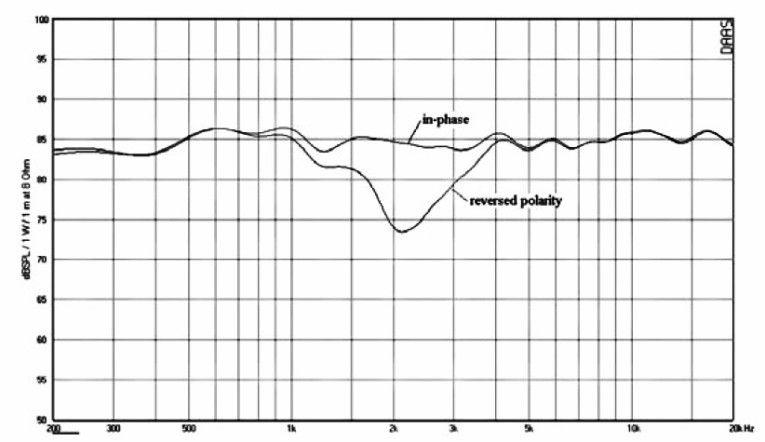
Comparing rise times, the woofer is approximately 250μs behind the tweeter. If you reverse the polarity of the tweeter, you get the step response shown in Fig. 20. There is now no longer a smooth transition from the tweeter to the woofer. The frequency response (Fig. 21) shows a null in the crossover region of about 12dB due to the tweeter polarity inversion. The response curves shown have been Z\n octave smoothed. The raw curve shows a notch of greater than 20dB, which is a strong indication that the drivers are in-phase at crossover. I will discuss this condition in more detail in the section on phase response.
Determining driver polarity can be of great value in home theater setups. For example, you may be using a center channel speaker from a different manufacturer than those of the right and left channels. If the center channel tweeter is connected out of phase to get flat frequency response while the left and right channel speakers use in-phase tweeters, you will degrade the imaging of the full system. The effect with woofers can be even more dramatic.
Phase Response
Recall that I did not list phase response as one of the predictors of loudspeaker preference. The vast majority of loudspeakers available today are not time coherent and therefore exhibit some degree of phase error. A great deal of research has gone into the subject of phase shift audibility. Papers in the AES and other audio journals are too numerous to reference.
Many researchers employed cascaded all-pass networks in the amplifying chain to introduce several hundred degrees of phase shift over the audible frequency range with no change in frequency magnitude response. The universal conclusion from these efforts is that large degrees of phase shift are not audible when listening to loudspeakers playing typical program material in the semi-reverberant environment of a typical listening room. Trained listeners using earphones have heard differences in sharp transient signals when subjected to very large frequency dependent phase shifts, but this is not the normal listening situation.
There is one possible exception to this conclusion. There is some evidence that large phase errors at low frequencies soften bass drum strikes. Loudspeakers develop large phase shifts near and below their low-end cutoff frequencies. This, in turn, produces group delays on the order of 5 to 15ms in that frequency range. Bass drum fundamentals then lag their upper harmonic components by this amount, which may explain this phenomenon. Countering this effect would require compensating bass amplitude and phase response flat down to below 10Hz or lower.
Notwithstanding the last three paragraphs, there are some things you can learn about a loudspeaker’s performance from phase data. Loudspeaker phase data is made up of two components: minimum phase and excess phase. The minimum phase response is related to the dips, peaks, and ripples in frequency magnitude response by a mathematical operation called the Hilbert transform. Any phase shift beyond this minimum phase shift is called excess phase, which is a measure of loudspeaker time dispersion. In particular, excess group delay, the derivative of excess phase with respect to frequency, has the units of time and is a measure of that dispersion.


DAAS measures total phase, computes minimum phase via the Hilbert transform, and then subtracts this from the total phase to get excess phase. DAAS then computes excess group delay from the excess phase. Figure 22 is a plot of the excess phase response for my example loudspeaker. The plot frequency range has been expanded to cover 500Hz to 20kHz. The excess phase starts out at about 30° and increases rapidly to almost 270° at 6kHz.
More revealing is the excess group delay shown in Fig. 23. Referring to the righthand scale, labeled “Delay/ms,” notice that excess group delay is essentially zero at high frequency. As you move down, the frequency axis toward the crossover point excess group delay begins to grow, reaching an asymptotic value of 0.25msec, or 250μsec, below 1000Hz. This confirms the estimate of the tweeter-woofer delay from the step response of Fig. 18. Excess group delay is an excellent tool for examining loudspeaker time dispersion.
Impedance
You can learn a great deal about a loudspeaker from its impedance plot. The impedance magnitude at low frequencies reflects the bass alignment of the speaker. For example, a sealed box speaker will have a single impedance peak at its low frequency resonance. Below this, frequency response will fall off at 12dB/octave. A vented enclosure will have a double peaked impedance plot at low frequencies. In this case the saddle point between the peaks approximates the vented box tuning frequency. (The woofer voice coil inductance and the crossover circuit may cause a slight shift in the saddle point relative to the actual box frequency.)
Below the box frequency the response of a vented speaker will fall at 24dB/octave. From fine detailed loudspeaker impedance curves you can detect cabinet vibrations and internal resonances such as standing waves. Finally, you can judge how difficult it will be for an amplifier to drive a particular loudspeaker. Very low impedance magnitude values coupled with large phase angles produce large current demands that may be beyond the capability of an amplifier.

Figures 24 and 25 are impedance plots for my example loudspeaker. Figure 24 covers the full frequency range. The minimum impedance of 6Ω occurs at 3kHz. The phase angle at this point is –22o. The worst phase angle occurs at 2kHz, but the impedance magnitude there is 10Ω. Driving this speaker should not be a problem for any well-designed amplifier.
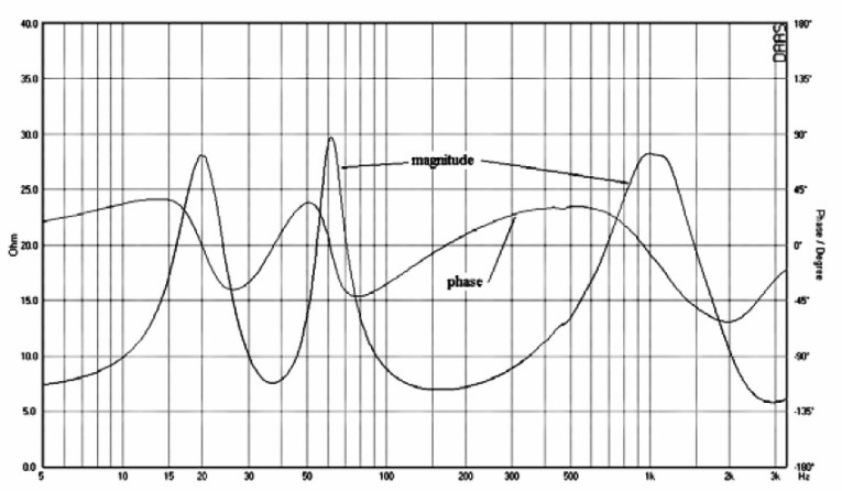
Figure 24 was generated at a 48kHz sample rate. Reducing the sample rate to 8kHz greatly improves low-frequency resolution. This is shown in Fig. 25. From this plot the tuning frequency, fB, is seen to be about 37Hz. In typical vented box alignments this is approximately the –6dB response level.
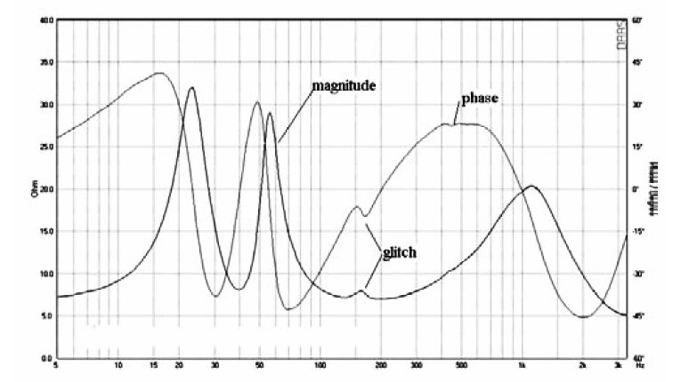
The impedance plot is also a diagnostic tool. Figure 26 is the impedance plot for a fairly well-regarded two-way tower loudspeaker. The impedance is shown on the same expanded scale as that of Fig. 25. Notice the glitch in both the magnitude and phase plots at 165Hz. There are three possible causes for this wrinkle in the impedance plot: port tube resonance, cabinet vibration, or a standing wave in the enclosure. Port tubes can develop organ pipe resonances. The port tube for this speaker is only about 15cm long, so I doubt port tube resonance is the cause because any organ pipe resonance would be much higher in frequency, but you can prove this rather simply.
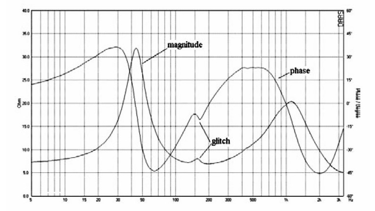
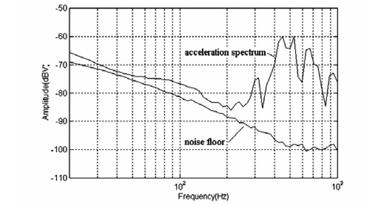
Figure 27 is an impedance plot of the speaker with the port tube plugged with a large block of polyfoam. Now there is the single peak characteristic of a sealed box alignment. But the glitch at 165Hz is still there and unchanged. So port resonance is not the
problem. Next side panel acceleration was measured with a Measurement Specialties ACH01 accelerometer driving the speaker with a 5V swept sine wave. The resulting acceleration spectrum is plotted in Fig. 28. Acceleration levels were so low I thought most of the measurement might just be accelerometer noise. So I measured the self-noise of the accelerometer, which is also plotted in Fig. 28.
Up to 200Hz acceleration levels are just slightly above the noise level. Acceleration peaks in the 400 to 500Hz range at about –60dBV, which translates into an acceleration level of about 0.14g. This may seem like a high level, but at 500Hz this amounts to a panel displacement of microns. More important, there is no acceleration spike at 165Hz. So panel vibration is not the problem.

This leaves the possibility of a standing wave. Figure 29 plots the low-frequency response of the tower speaker. This plot was obtained using the previously described feature in DAAS for combining near-field woofer and port outputs. This plot is valid up to about 300Hz. Notice the small dip at 165Hz, which represents the power taken from the woofer output to sustain a standing wave within the enclosure.
Now I could have guessed the problem was a standing wave from the beginning if I had first described the physical appearance of the speaker, but I wanted to highlight the analytical tools available to examine this problem. The tower internal height is 102cm. The woofer is mounted at the top of the front baffle. So you have a closed pipe excited at one end. Assuming a sound velocity of 343m/sec, this calculates out to a standing wave at 168Hz. Given a small amount of filling material which may slow sound speed in the enclosure, 165Hz seems right on.
Efficiency And Sensitivity
A loudspeaker’s efficiency tells you how much acoustic power and sound pressure level a loudspeaker can produce for each electrical watt of input power. It is specified in terms of the sound pressure level generated with 1W input at a distance of 1m, i.e. dBspl/1W/1m. Because loudspeaker impedance varies widely over frequency both in magnitude and phase, it is difficult to determine the true input power to a loudspeaker. To get around this problem a constant resistance is assumed for the loudspeaker impedance.
Typically a value of either 4 or 8Ω is used. The assumption of a constant resistive impedance in the efficiency measurement means that frequency response tests which are nominally made with constant input power are actually made with a constant input voltage. Modern solid-state amplifiers are essentially constant voltage sources. As long as output stage current limits are not reached, these amplifiers will provide whatever current is required to meet the demands of the constant voltage frequency sweep. For this reason it is now common practice to specify loudspeaker performance in terms of voltage sensitivity, S0, which has the units of
dBspl/2.83V/1m.
2.83V represents the voltage that will produce 1W of power dissipation in an 8Ω resistor.
I have measured hundreds of loudspeakers for sensitivity. In my tests values have ranged from 84 to 91dB. All other things being equal, the higher the sensitivity the better. Unfortunately, all other things are rarely equal. Speakers with the smoothest frequency response are often not the most sensitive.
As part of the frequency response measurement, DAAS calculates the distance from the microphone to the loudspeaker under test and automatically references the measurement to 1m. I then calculate sensitivity as the mean SPL over the 500Hz to 2kHz band. Looking at Fig. 3 in part 1, the sensitivity of my example speaker is 85dBspl/2.83V/1m.
Distortion
First, you must distinguish between linear and nonlinear distortion. If a loudspeaker is linear, doubling an electrical input signal will exactly double its acoustic output. If two frequencies, f1 and f2, are input to a linear loudspeaker, only those two frequencies and no other frequencies will appear in the output. Any departure from flat frequency response will distort a signal. This is linear amplitude distortion.
The relative magnitudes of f1 and f2 may change, but no additional frequencies are produced. On the other hand, nonlinear distortions such as harmonic and intermodulation distortion produce signal components not in the original program
material.
I have not found a quantitative or qualitative relationship between the various distortion types you can easily measure and loudspeaker preference. The audibility of nonlinear distortion is a complicated issue. It is relatively easy to detect a few percent distortion in simple signals such as a pair of sine waves. However, large levels of distortion can be tolerated in complex program material such as rock ‘n’ roll music. In my experience, the maximum sound pressure level a speaker can generate is dictated by the level of distortion the listener will tolerate.
Distortion measurements do not directly predict how a speaker will sound, rather they help us judge driver linearity and by implication driver quality. DAAS implements tests for harmonic and intermodulation distortion. Although I will show some harmonic distortion test results, I believe that intermodulation distortion tests are more revealing of loudspeaker performance.
We can tolerate relatively high levels of harmonic distortion in program material because, as their name implies, the spurious components added to the program are harmonically related to the original program. Intermodulation distortion (IMD) produces output frequencies that are not harmonically related to the input. These frequencies are much more audible and annoying than harmonic distortion. In one kind of IMD test two frequencies are input to the speaker. Let the symbols f1 and f2 represent the two frequencies used in the test. Then a 2nd-order nonlinearity will produce intermods at frequencies of f1 ± f2. A 3rd-order nonlinearity generates intermods at 2f1 ± f2 and f1 ± 2f2.
I ran a harmonic distortion test on my example loudspeaker. Average level was set at 90dB/1m. Figure 30 plots the 3rd and 5th harmonic distortion levels out to 8kHz. The test consists of a sequence of 50 distinct frequencies from 100Hz to 8kHz. Only the odd-order distortion products are shown because these are known to be most objectionable.
Distortion components average about 0.32% up to 300Hz and drop to below 0.1% beyond that point. The one outlier of 1% at 180Hz is a false reading caused by a panel vibration in my lab interfering with the speaker output at the mike location. Apparently the resonant frequency of this panel aligns almost perfectly with test frequency of 180Hz.
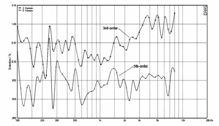
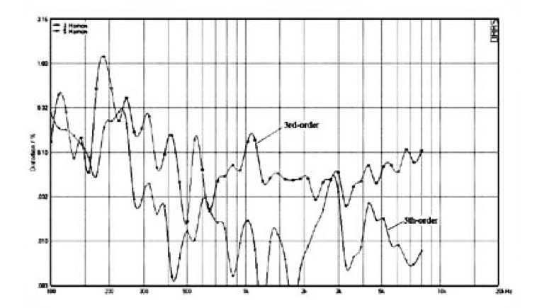
Figure 31 shows the results for the same test run on the PA speaker at an average level of 87dB/1m. (Distortion was excessively high at 90dB/1m.) Notice that tweeter 3rd harmonic distortion rises to 1% above 3kHz. The 5th–order distortion averages 0.32% above 300Hz. It is clear that the drivers used in the PA speaker are of poorer quality than those used in my example speaker.
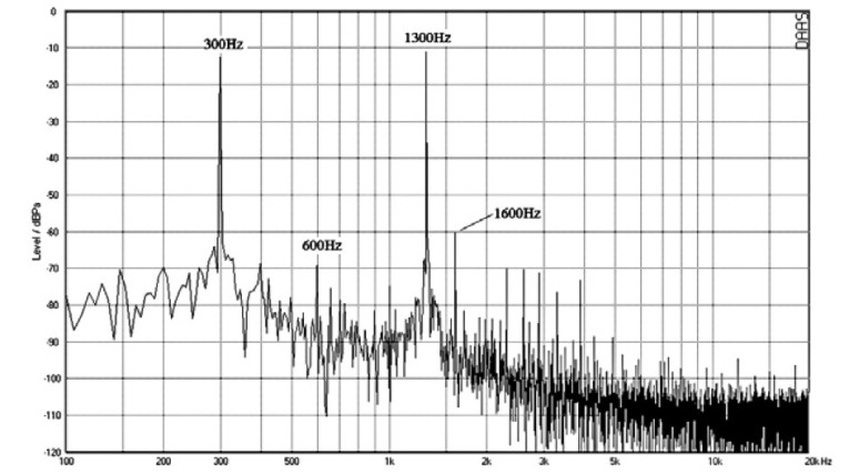
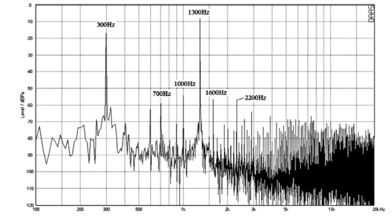
Next I examined IMD in the woofers. Figure 32 shows results for the two-tone IMD test run on my example speaker at the 90dBspl level. The two frequencies of 300 and 1300Hz were picked to exercise the woofer. There is a 2nd-harmonic of the 300Hz tone at 600Hz, but it is down 60dB from 300Hz. The only significant IM product is a 2nd-order one at 1600Hz. It is down 56dB from the full output. The same test was then run on the PA speaker. Examining Fig. 33, you can see significant IM products at 700, 1000, 1600, and 2200Hz.
Dynamics
How often have you turned up the volume only to feel that the music is not getting louder? The sound stage seems to collapse, transients dull, and the sound becomes congested and lifeless. You are experiencing short-term dynamic compression. You
have exceeded the SPL capability of your loudspeaker. When listening to classical music, short-term transients may exceed the average sound level by 12 to 20dB. If the program material increases by 12dB, but your speaker output only increases by 10dB, you are experiencing dynamic compression.
Short-term dynamic compression should not be confused with power compression. In sound reinforcement applications such as rock concerts, the average power level fed to the loudspeakers is quite high. Under this condition driver voice coils heat up. The coil resistance increases, reducing the driver sensitivity. This is power compression.
In typical home listening environments, average power levels are only a few watts at most. Voice coil heating is not much of a problem. In this case the compression arises out of some nonlinear behavior of the driver compliance or magnetic field distribution such that the driver cone excursion does not keep up with the input voltage demand.

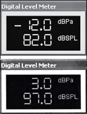
DAAS has many interesting signals in its signal library that can be used to test loudspeaker dynamic response. One signal consists of a set of eight sine waves spread out over an interval from 500Hz to 2.5kHz. The spectrum of this signal is shown in Fig. 34. This signal can be played as a single event and the resulting SPL measured. Then the signal can be quickly increased by several dB and played again.
Summary
We have seen that the single best predictor of loudspeaker listener preference is frequency response. There are four elements to frequency response: on-axis response, listening window response, early reflection response and, finally, power response. The last two require that you also examine polar response. Resonances are the principle causes of objectionable sound. Strong resonances are often obvious in the frequency response plots. However, the CSD and PCSD provide us with more detail and often reveal delayed resonances not obvious in the frequency response alone.
Turning to the time domain, the step response gives us qualitative information on driver polarity, time dispersion, and driver integration. Phase response is not a strong indicator of speaker quality, but we can glean more detailed information on speaker time dispersion from the excess group delay plot.
Impedance data can be used to detect cabinet vibrations and internal resonances such as standing waves. We can also judge how difficult it will be for an amplifier to drive a particular loudspeaker. Very low impedance magnitude values coupled with large phase angles produce large current demands that may be beyond the capability of an amplifier.
Unless distortion levels are very high, harmonic and IM distortions are not strong predictors of listener preference, but they are useful in assessing driver quality and can explain why speakers sound bad when played at high volume levels. The dynamic capability of a loudspeaker is a very strong predictor of its ability to produce lifelike sound. Finally, the measurements discussed here are not only useful in evaluating existing designs, but they can also be used by loudspeaker engineers as design goals.
There is one caveat in all these results. The discussions here have been limited to conventional, forward-firing dynamic loudspeaker systems. Large panel loudspeakers and line arrays present vastly different measurement challenges. In the home listening environment, you will invariably be in the near field of these speaker types. Response will vary widely with listener position in height and distance to the speaker. Defining a single response axis that characterizes one of these speakers is difficult. Also, polar response will differ substantially from conventional speakers. aX
A note on testing
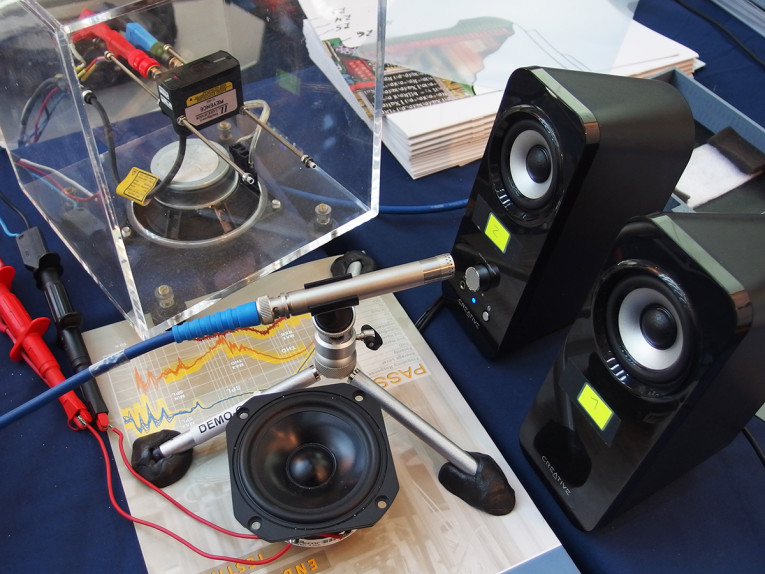
All measurements used in this article were made with either the DAAS4usb or the DAAS4pro192 PC-controlled acoustic data acquisition and analysis systems. Acoustic data was measured with either a calibrated Earthworks MD30 microphone or ACO Pacific 7012 ½″ laboratory grade condenser microphone and a custom designed wide-band, low-noise preamp. Cabinet vibration was measured with a Measurement Specialties ACH01 accelerometer. Polar response tests were performed with a computer-controlled OUTLINE turntable.
This article was originally published in audioXpress, October 2008
Read Part 1 of this article here.